Predicting Stroke
1 Introduction
1.1 Overview
According to the World Health Organization (WHO) stroke is the 2nd leading cause of death globally, responsible for approximately 11% of total deaths. Six and a half-million people die from stroke annually(3.3 million from ischaemic stroke annually, 2.9 million from intracerebral haemorrhages and 0.3 million from subarachnoid haemorrhages). One in four people over age 25 will have a stroke in their lifetime. 62% of all incident strokes are ischaemic strokes while 28% are intracerebral haemorrhages and 10% are subarachnoid haemorrhages.
1.2 About the Data
This data set is used to predict whether a patient is likely to get stroke based on some input parameters like gender, age, hypertension, heart diseases, residence, bmi and smoking status. Each row in the data provides relevant information about the patient.
The data dictionary is as follows:
- id: unique identifier
- gender: “Male”, “Female” or “Other”
- age: age of the patient
- hypertension: 0 if the patient doesn’t have hypertension, 1 if the patient has hypertension
- heart_disease: 0 if the patient doesn’t have any heart diseases, 1 if the patient has a heart disease
- ever_married: “No” or “Yes”
- work_type: “children”, “Govt_jov”, “Never_worked”, “Private” or “Self-employed”
- Residence_type: “Rural” or “Urban”
- avg_glucose_level: average glucose level in blood
- bmi: body mass index
- smoking_status: “formerly smoked”, “never smoked”, “smokes” or “Unknown”*
- stroke: 1 if the patient had a stroke or 0 if not
*Note: “Unknown” in smoking_status means that the information is unavailable for this patient
2 Data Exploration
2.1 loading Relevant packages
#Import relevant packages

library(tidyverse)
library(janitor)
library(readr)
library(plotly)
library(knitr)
2.2 loading Data Set
stroke <- read_csv('https://raw.githubusercontent.com/reinpmomz/Data_sets/main/Data/healthcare-dataset-stroke-data.csv', na=c("N/A"))%>%
clean_names()rmarkdown::paged_table(stroke)dim(stroke)## [1] 5110 12- Our data has 5110 observations and 12 variables
##checking the data structure

str(stroke)
## spc_tbl_ [5,110 x 12] (S3: spec_tbl_df/tbl_df/tbl/data.frame)
## $ id : num [1:5110] 9046 51676 31112 60182 1665 ...
## $ gender : chr [1:5110] "Male" "Female" "Male" "Female" ...
## $ age : num [1:5110] 67 61 80 49 79 81 74 69 59 78 ...
## $ hypertension : num [1:5110] 0 0 0 0 1 0 1 0 0 0 ...
## $ heart_disease : num [1:5110] 1 0 1 0 0 0 1 0 0 0 ...
## $ ever_married : chr [1:5110] "Yes" "Yes" "Yes" "Yes" ...
## $ work_type : chr [1:5110] "Private" "Self-employed" "Private" "Private" ...
## $ residence_type : chr [1:5110] "Urban" "Rural" "Rural" "Urban" ...
## $ avg_glucose_level: num [1:5110] 229 202 106 171 174 ...
## $ bmi : num [1:5110] 36.6 NA 32.5 34.4 24 29 27.4 22.8 NA 24.2 ...
## $ smoking_status : chr [1:5110] "formerly smoked" "never smoked" "never smoked" "smokes" ...
## $ stroke : num [1:5110] 1 1 1 1 1 1 1 1 1 1 ...
## - attr(*, "spec")=
## .. cols(
## .. id = col_double(),
## .. gender = col_character(),
## .. age = col_double(),
## .. hypertension = col_double(),
## .. heart_disease = col_double(),
## .. ever_married = col_character(),
## .. work_type = col_character(),
## .. Residence_type = col_character(),
## .. avg_glucose_level = col_double(),
## .. bmi = col_double(),
## .. smoking_status = col_character(),
## .. stroke = col_double()
## .. )
## - attr(*, "problems")=<externalptr>From the output on the data structure, all of the data has been read as numeric values(‘double’ value or a decimal type with at least two decimal places) and character values but some should be converted to factors since they are categorical.
2.3 Converting into factors
stroke_final <- stroke%>%
  filter(gender!= "Other")%>%
  mutate(gender = factor(gender, levels = c("Female", "Male")))%>%
  mutate(hypertension= factor(hypertension, levels = c(0,1),
                                      labels = c("No", "Yes")))%>%
  mutate(heart_disease= factor(heart_disease, levels = c(0,1),
                                      labels = c("No", "Yes")))%>%
  mutate(ever_married = factor(ever_married, levels = c("No", "Yes")))%>%
  mutate(across(c(work_type, residence_type, smoking_status), as.factor))%>%
  mutate(stroke= factor(stroke, levels = c(0,1),
                                      labels = c("No", "Yes")))%>%
  labelled::set_variable_labels(
    id = "unique identifier",
  gender = "Sex of the patient",
  age = "Age of the patient",
  hypertension = "Patient has hypertension",
  heart_disease = "Patient has heart disease",
  ever_married = "Patient is married",
  work_type = "Work type",
  residence_type = "Residence type",
  avg_glucose_level = "Average glucose level in blood",
  bmi = "Body mass index (in kg/m2)",
  smoking_status = "Smoking status",
  stroke = "Patient had stroke"
  )
2.4 checking missing values
sum(is.na(stroke_final))## [1] 201#which(is.na(stroke_final))
#which(!complete.cases(stroke_final))
sapply(stroke_final,function(x) sum(is.na(x)))## id gender age hypertension
## 0 0 0 0
## heart_disease ever_married work_type residence_type
## 0 0 0 0
## avg_glucose_level bmi smoking_status stroke
## 0 201 0 0There were 201 missing values in bmi variable in our data set.
3 Exploratory data analysis
3.1 Univariate analysis
This is analysis of one variable to enable us understand the distribution of values for a single variable.
3.1.1 Normality of continous variables
shapiro.test(stroke_final$bmi)##
## Shapiro-Wilk normality test
##
## data: stroke_final$bmi
## W = 0.95357, p-value < 2.2e-16The shapiro.test has a restriction in R that it can be applied only up to a sample of size 5000 and the least sample size must be 3. Therefore, we have an alternative hypothesis test called Anderson Darling normality test. To perform this test, we need load nortest package and use the ad.test function
nortest::ad.test(stroke_final$age)##
## Anderson-Darling normality test
##
## data: stroke_final$age
## A = 33.876, p-value < 2.2e-16nortest::ad.test(stroke_final$avg_glucose_level)##
## Anderson-Darling normality test
##
## data: stroke_final$avg_glucose_level
## A = 352.33, p-value < 2.2e-16If the p-value < 0.05, it implies that the distribution of the data are significantly different from normal distribution. In other words, we cannot assume the normality.
3.1.2 Descriptives Frequency table
library(gtsummary)
library(flextable)

set_gtsummary_theme(list(
  "tbl_summary-fn:percent_fun" = function(x) style_percent(x, digits = 1),
  "tbl_summary-str:categorical_stat" = "{n} ({p}%)"
))
# Setting `Compact` theme
theme_gtsummary_compact()
# make dataset with variables to summarize
tbl_summary(stroke_final%>%
dplyr::select(-id),
type = list(
all_dichotomous() ~ "categorical",
all_continuous() ~ "continuous2")
, statistic = all_continuous() ~ c(
"{mean} ({sd})",
"{median} ({p25}, {p75})",
"{min}, {max}")
, digits = all_continuous() ~ 2
, missing = "always" # don't list missing data separately
,missing_text = "Missing"
) %>%
modify_header(label = "**Descriptives**") %>% # update the column header
bold_labels() %>%
italicize_levels()%>%
add_n() # add column with total number of non-missing observations| Descriptives | N | N = 5,1091 |
|---|---|---|
| Sex of the patient | 5,109 | |
| Female | 2,994 (58.6%) | |
| Male | 2,115 (41.4%) | |
| Missing | 0 | |
| Age of the patient | 5,109 | |
| Mean (SD) | 43.23 (22.61) | |
| Median (IQR) | 45.00 (25.00, 61.00) | |
| Range | 0.08, 82.00 | |
| Missing | 0 | |
| Patient has hypertension | 5,109 | |
| No | 4,611 (90.3%) | |
| Yes | 498 (9.75%) | |
| Missing | 0 | |
| Patient has heart disease | 5,109 | |
| No | 4,833 (94.6%) | |
| Yes | 276 (5.40%) | |
| Missing | 0 | |
| Patient is married | 5,109 | |
| No | 1,756 (34.4%) | |
| Yes | 3,353 (65.6%) | |
| Missing | 0 | |
| Work type | 5,109 | |
| children | 687 (13.4%) | |
| Govt_job | 657 (12.9%) | |
| Never_worked | 22 (0.43%) | |
| Private | 2,924 (57.2%) | |
| Self-employed | 819 (16.0%) | |
| Missing | 0 | |
| Residence type | 5,109 | |
| Rural | 2,513 (49.2%) | |
| Urban | 2,596 (50.8%) | |
| Missing | 0 | |
| Average glucose level in blood | 5,109 | |
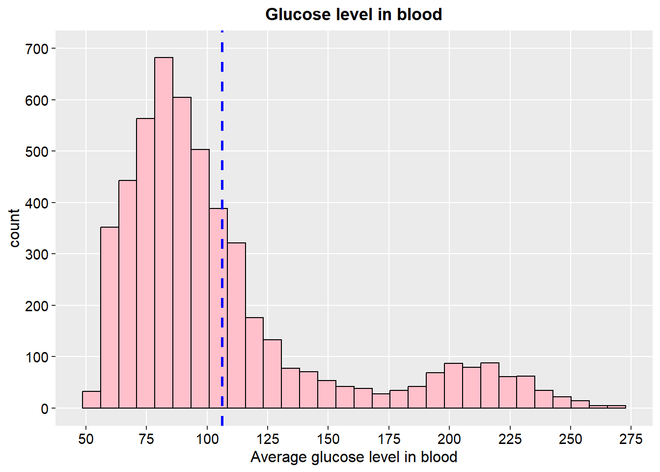
| Mean (SD) | 106.14 (45.29) | |
| Median (IQR) | 91.88 (77.24, 114.09) | |
| Range | 55.12, 271.74 | |
| Missing | 0 | |
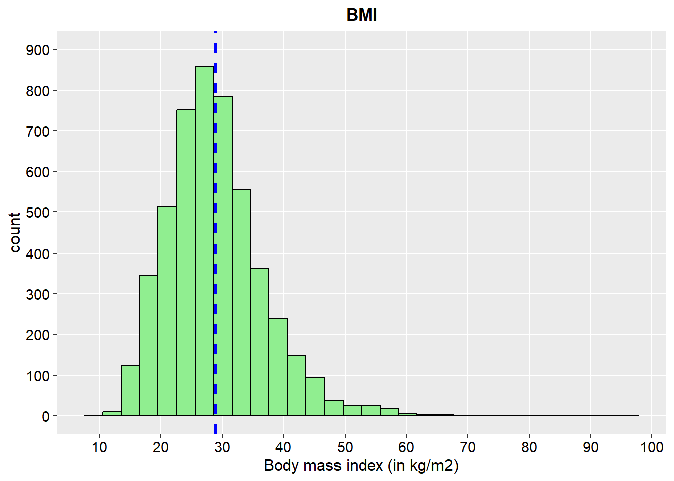
| Body mass index (in kg/m2) | 4,908 | |
| Mean (SD) | 28.89 (7.85) | |
| Median (IQR) | 28.10 (23.50, 33.10) | |
| Range | 10.30, 97.60 | |
| Missing | 201 | |
| Smoking status | 5,109 | |
| formerly smoked | 884 (17.3%) | |
| never smoked | 1,892 (37.0%) | |
| smokes | 789 (15.4%) | |
| Unknown | 1,544 (30.2%) | |
| Missing | 0 | |
| Patient had stroke | 5,109 | |
| No | 4,860 (95.1%) | |
| Yes | 249 (4.87%) | |
| Missing | 0 | |
| 1 n (%) | ||
3.1.3 Visualization
library(ggpubr)


 ggplot(stroke_final, aes(x=stroke))+
  geom_bar(aes(fill = stroke), show.legend = FALSE)+
  labs(x="",y="", title = "Patient had stroke")+
  geom_text(aes(label = paste0(..count.., " (", scales::percent(after_stat(prop), accuracy = .1), ")"), group=1),
            stat = "count", vjust = 1.1, colour = "black")+
  #guides(fill = FALSE)+
  theme_pubclean()+
  theme(axis.title = element_text(face="bold",color="black",size=13),
        #legend.position = "none",
        axis.text.y = element_text(color="black",size=12),
        axis.text.x = element_text(color="black",size=11),
        plot.title = element_text(hjust = 0.5, face="bold",color="black",size=13),
        panel.grid.major.x = element_blank())


 ggplot(stroke_final, aes(x=gender))+
  geom_bar(aes(fill = gender), show.legend = FALSE)+
  labs(x="",y="", title = "Sex of the patient")+
  scale_y_continuous(breaks = seq(0, 3000, by = 500), limits = c(0, 3000))+
  theme_pubclean()+
  geom_text(aes(label = paste0(after_stat(count), " (", scales::percent(after_stat(prop), accuracy = .01), ")"), group=1),
            stat = "count", vjust = -0.4, colour = "black")+
  theme(axis.title = element_text(face="bold",color="black",size=13),
        axis.text = element_text(color="black",size=12),
        plot.title = element_text(hjust = 0.5, face="bold",color="black",size=13),
        panel.grid.major.x = element_blank())

 ggplot(stroke_final, aes(x=hypertension))+
  geom_bar(aes(fill = hypertension), show.legend = FALSE)+
  labs(x="",y="", title = "Patient has hypertension")+
  scale_y_continuous(breaks = seq(0, 5000, by = 1000), limits = c(0, 5000))+
  theme_pubclean()+
  geom_text(aes(label = paste0(after_stat(count), " (", scales::percent(after_stat(prop), accuracy = .1), ")"), group=1),
            stat = "count", vjust = 1.1, colour = "black")+
  theme(axis.title = element_text(face="bold",color="black",size=13),
        axis.text = element_text(color="black",size=12),
        plot.title = element_text(hjust = 0.5, face="bold",color="black",size=13),
        panel.grid.major.x = element_blank())

 ggplot(stroke_final, aes(x=heart_disease))+
  geom_bar(aes(fill = heart_disease), show.legend = FALSE)+
  labs(x="",y="", title = "Patient has heart disease")+
  scale_y_continuous(breaks = seq(0, 5000, by = 1000), limits = c(0, 5000))+
  theme_pubclean()+
  geom_text(aes(label = paste0(after_stat(count), " (", scales::percent(after_stat(prop), accuracy = .1), ")"), group=1),
            stat = "count", vjust = 1.1, colour = "black")+
  theme(axis.title = element_text(face="bold",color="black",size=13),
        axis.text.y = element_text(color="black",size=12),
        axis.text.x = element_text(color="black",size=12, angle = 0),
        plot.title = element_text(hjust = 0.5, face="bold",color="black",size=13),
        panel.grid.major.x = element_blank())


 ggplot(stroke_final, aes(x=ever_married))+
  geom_bar(aes(fill = ever_married), show.legend = FALSE)+
  labs(x="",y="", title = "Patient is married")+
  scale_y_continuous(breaks = seq(0, 3500, by = 500), limits = c(0, 3500))+
 theme_pubclean()+
  geom_text(aes(label = paste0(after_stat(count), " (", scales::percent(after_stat(prop), accuracy = .1), ")"), group=1),
            stat = "count", vjust = 1.1, colour = "black")+
  theme(axis.title= element_text(face="bold",color="black",size=13),
        axis.text = element_text(color="black",size=12),
        plot.title = element_text(hjust = 0.5, face="bold",color="black",size=13),
        panel.grid.major.x = element_blank())


 ggplot(stroke_final, aes(x=work_type))+
  geom_bar(aes(fill = work_type), show.legend = FALSE)+
  labs(x="",y="", title = "Work type")+
  scale_y_continuous(breaks = seq(0, 3100, by = 500), limits = c(0, 3100))+
  theme_pubclean()+
  geom_text(aes(label = paste0(after_stat(count), " (", scales::percent(after_stat(prop), accuracy = .1), ")"), group=1),
            stat = "count", vjust = -0.4, colour = "black")+
  theme(axis.title = element_text(face="bold",color="black",size=13),
        axis.text.y = element_text(color="black",size=12),
        axis.text.x = element_text(color="black",size=11, angle = 0),
        plot.title = element_text(hjust = 0.5, face="bold",color="black",size=13),
        panel.grid.major.x = element_blank())


 ggplot(stroke_final, aes(x=residence_type))+
  geom_bar(aes(fill = residence_type), show.legend = FALSE)+
  labs(x="",y="", title = "Residence type")+
  scale_y_continuous(breaks = seq(0, 2800, by = 400), limits = c(0, 2800))+
  theme_pubclean()+
  geom_text(aes(label = paste0(after_stat(count), " (", scales::percent(after_stat(prop), accuracy = .1), ")"), group=1),
            stat = "count", vjust = 1.5, colour = "black")+
  theme(axis.title = element_text(face="bold",color="black",size=13),
        axis.text = element_text(color="black",size=12),
        plot.title = element_text(hjust = 0.5, face="bold",color="black",size=13),
        panel.grid.major.x = element_blank())


 ggplot(stroke_final, aes(x=smoking_status))+
  geom_bar(aes(fill = smoking_status), show.legend = FALSE)+
  labs(x="",y="", title = "Smoking status")+
  scale_y_continuous(breaks = seq(0, 2000, by = 400), limits = c(0, 2000))+
  theme_pubclean()+
  geom_text(aes(label = paste0(after_stat(count), " (", scales::percent(after_stat(prop), accuracy = .1), ")"), group=1),
            stat = "count", vjust = 1.5, colour = "black")+
  theme(axis.title = element_text(face="bold",color="black",size=13),
        axis.text.y = element_text(color="black",size=12),
        axis.text.x = element_text(color="black",size=11, angle = 0),
        plot.title = element_text(hjust = 0.5, face="bold",color="black",size=13),
        panel.grid.major.x = element_blank())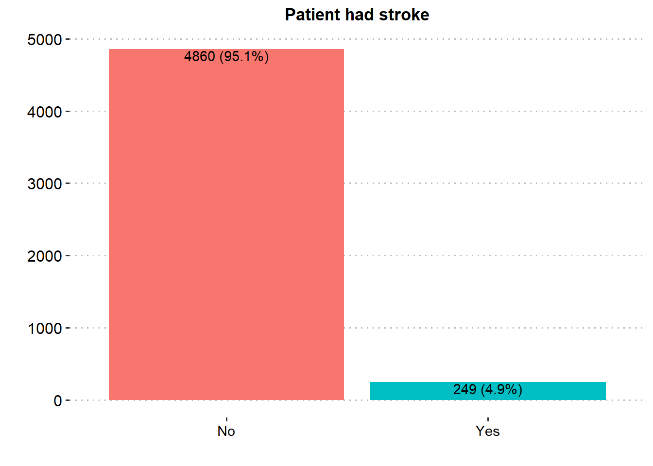
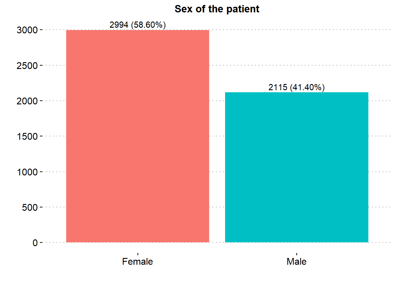
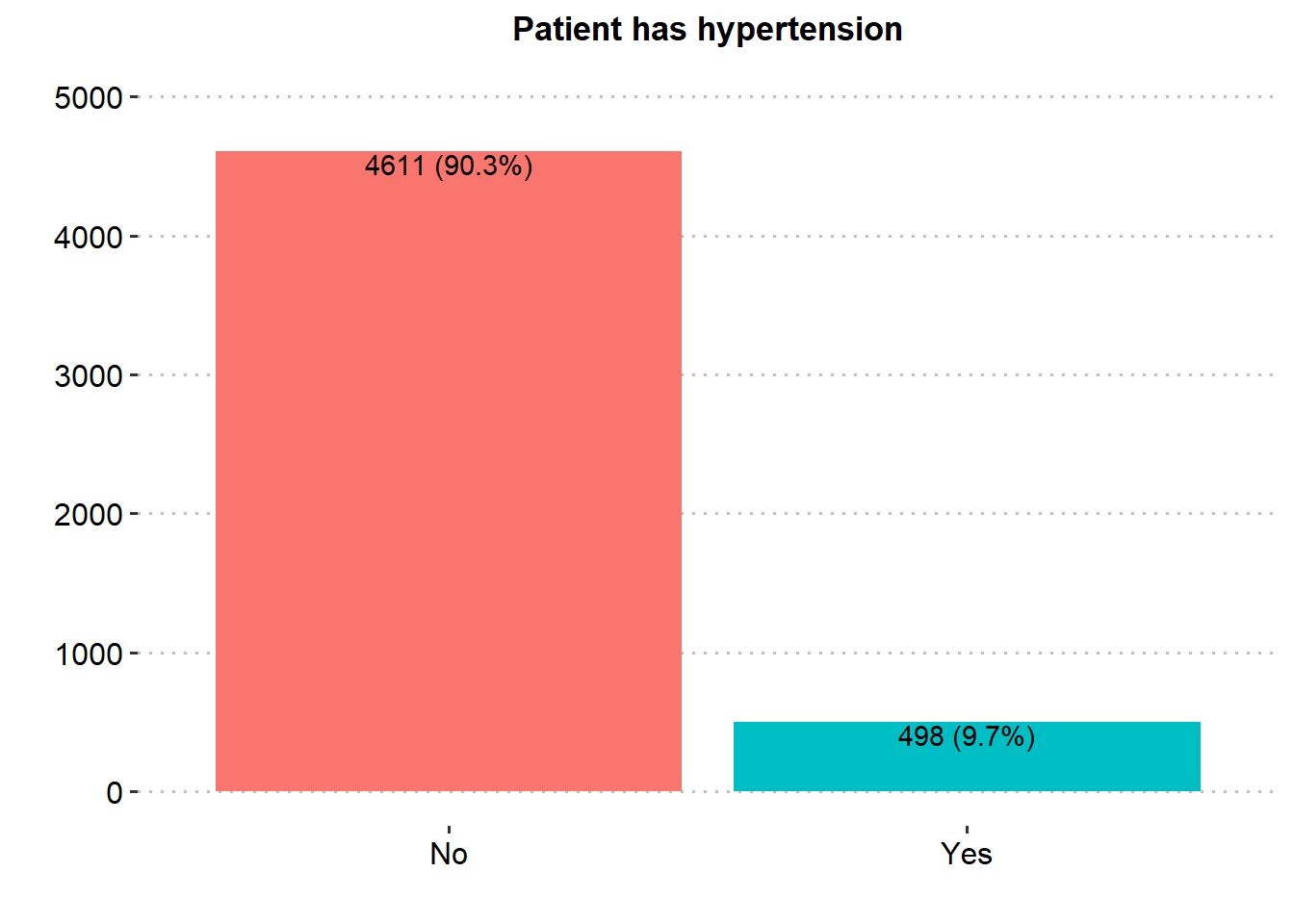
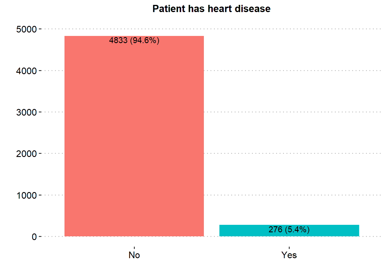
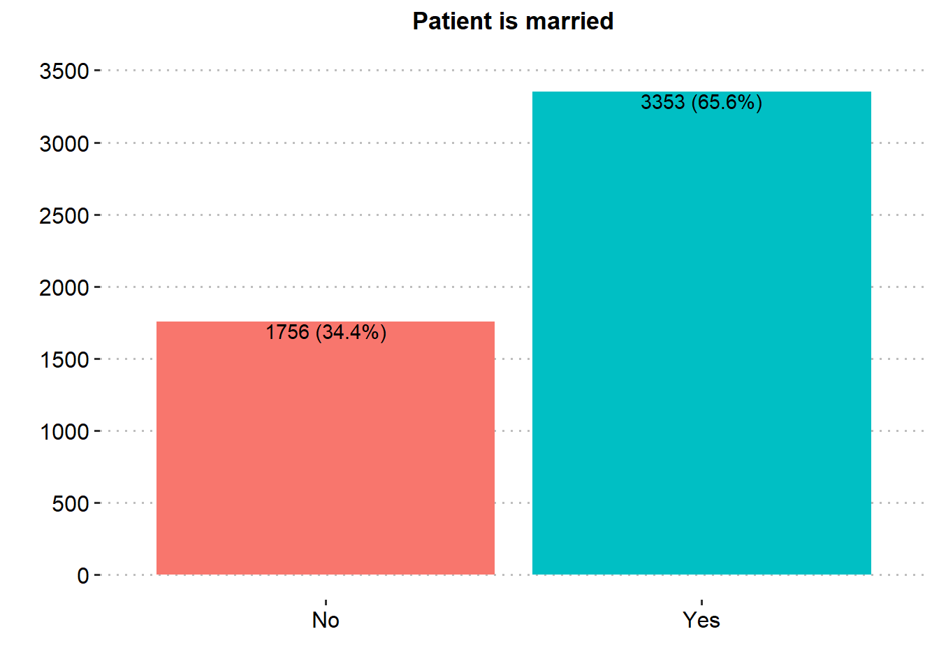
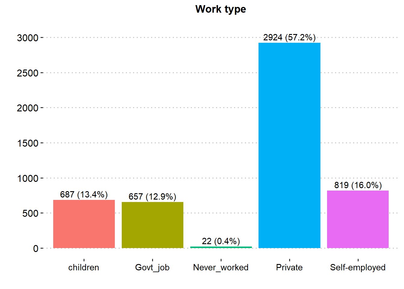
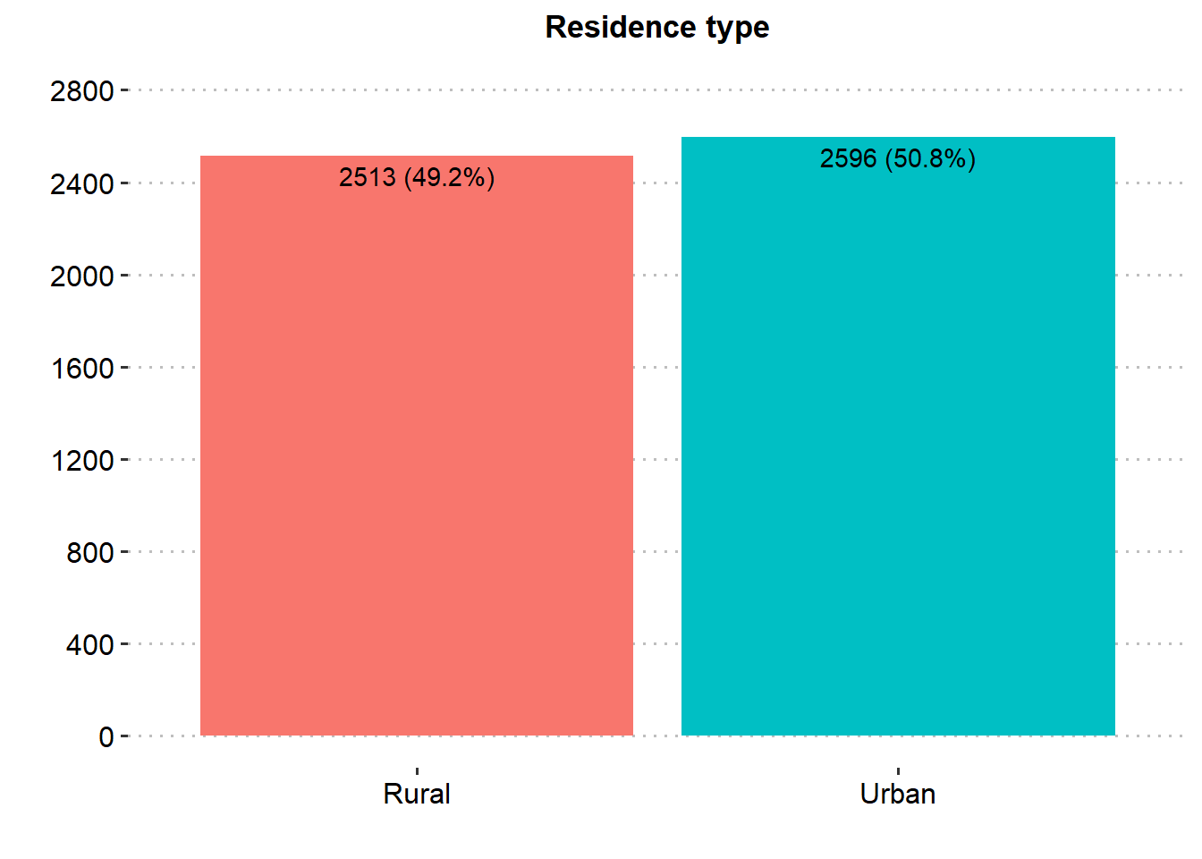
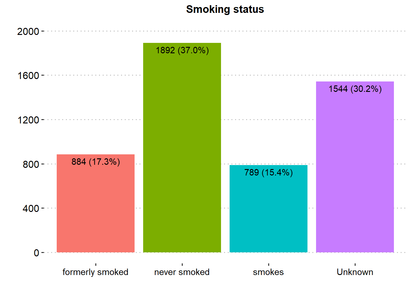
Majority of the patients were Female (58.6%), married (65.6%), in private employment (57.2%), had no hypertension (90.3%), had no heart disease (94.6%) and had never smoked (37.0%). There was similar proportion in rural and urban residence type.
ggplot(stroke_final, aes(x=age)) +
  geom_histogram(color="black", fill="lightblue")+
  geom_vline(aes(xintercept=mean(age)),
            color="blue", linetype="dashed", size=1)+
   scale_y_continuous(breaks = seq(0, 300, by = 50), limits = c(0, 300))+
  scale_x_continuous(n.breaks = 10)+
  labs(x="Age of the Patient",y="count", title = "Age (Years)")+
  theme(axis.title = element_text(color="black",size=12),
        axis.text = element_text(color="black",size=11),
        plot.title = element_text(hjust = 0.5, face="bold",color="black",size=13),
        panel.grid.minor.y = element_blank(),
        panel.grid.minor.x = element_blank())

ggplot(stroke_final, aes(x=avg_glucose_level)) +
  geom_histogram(color="black", fill="pink")+
  geom_vline(aes(xintercept=mean(avg_glucose_level)),
            color="blue", linetype="dashed", size=1)+
  scale_y_continuous(breaks = seq(0, 700, by = 100), limits = c(0, 700))+
  scale_x_continuous(n.breaks = 12)+
  labs(x="Average glucose level in blood",y="count", title = "Glucose level in blood")+
  theme(axis.title = element_text(color="black",size=12),
        axis.text = element_text(color="black",size=11),
        plot.title = element_text(hjust = 0.5, face="bold",color="black",size=13),
        panel.grid.minor.y = element_blank(),
        panel.grid.minor.x = element_blank())

ggplot(stroke_final%>%
         drop_na(bmi), aes(x=bmi)) +
  geom_histogram(color="black", fill="lightgreen")+
  geom_vline(aes(xintercept=mean(bmi)),
            color="blue", linetype="dashed", size=1)+
    scale_y_continuous(breaks = seq(0, 900, by = 100), limits = c(0, 900))+
  scale_x_continuous(n.breaks = 10)+
  labs(x="Body mass index (in kg/m2)",y="count", title = "BMI")+
  theme(axis.title = element_text(color="black",size=12),
        axis.text = element_text(color="black",size=11),
        plot.title = element_text(hjust = 0.5, face="bold",color="black",size=13),
        panel.grid.minor.y = element_blank(),
        panel.grid.minor.x = element_blank())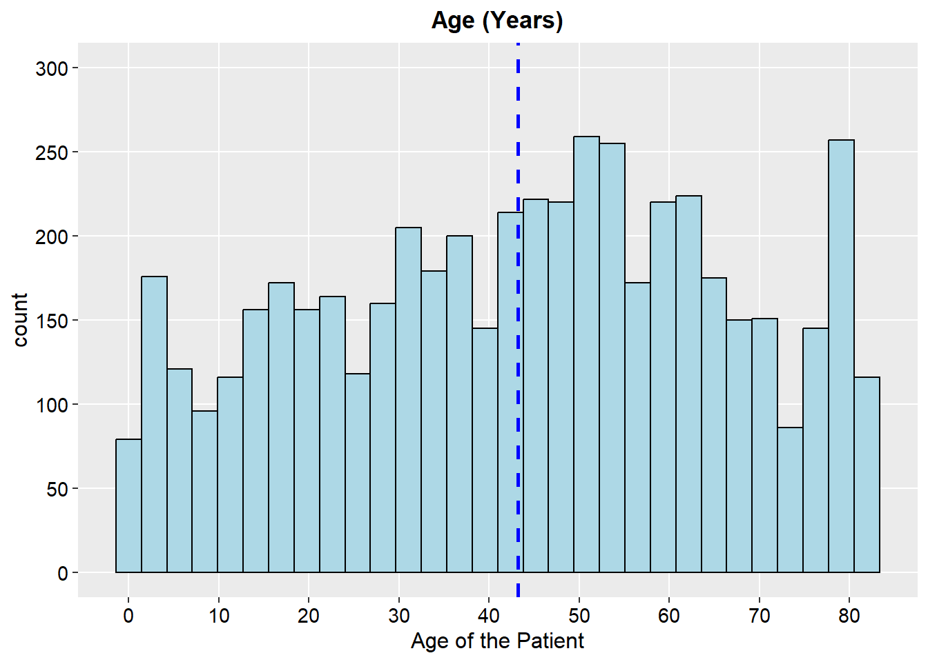
3.2 Bivariate analysis
3.2.1 Correlation
Pearson correlation evaluates the linear relationship between two continuous variables.
# improved correlation matrix
library(corrplot)

corrplot(cor(stroke_final%>%
               dplyr::select(-id)%>%
               mutate(across(c(1:11), as.numeric)),
             method='pearson', use = "complete.obs"),
  method = "color", #number
  addCoef.col = "black",
  number.cex = 0.95,
  type = "upper" # show only upper side #full
)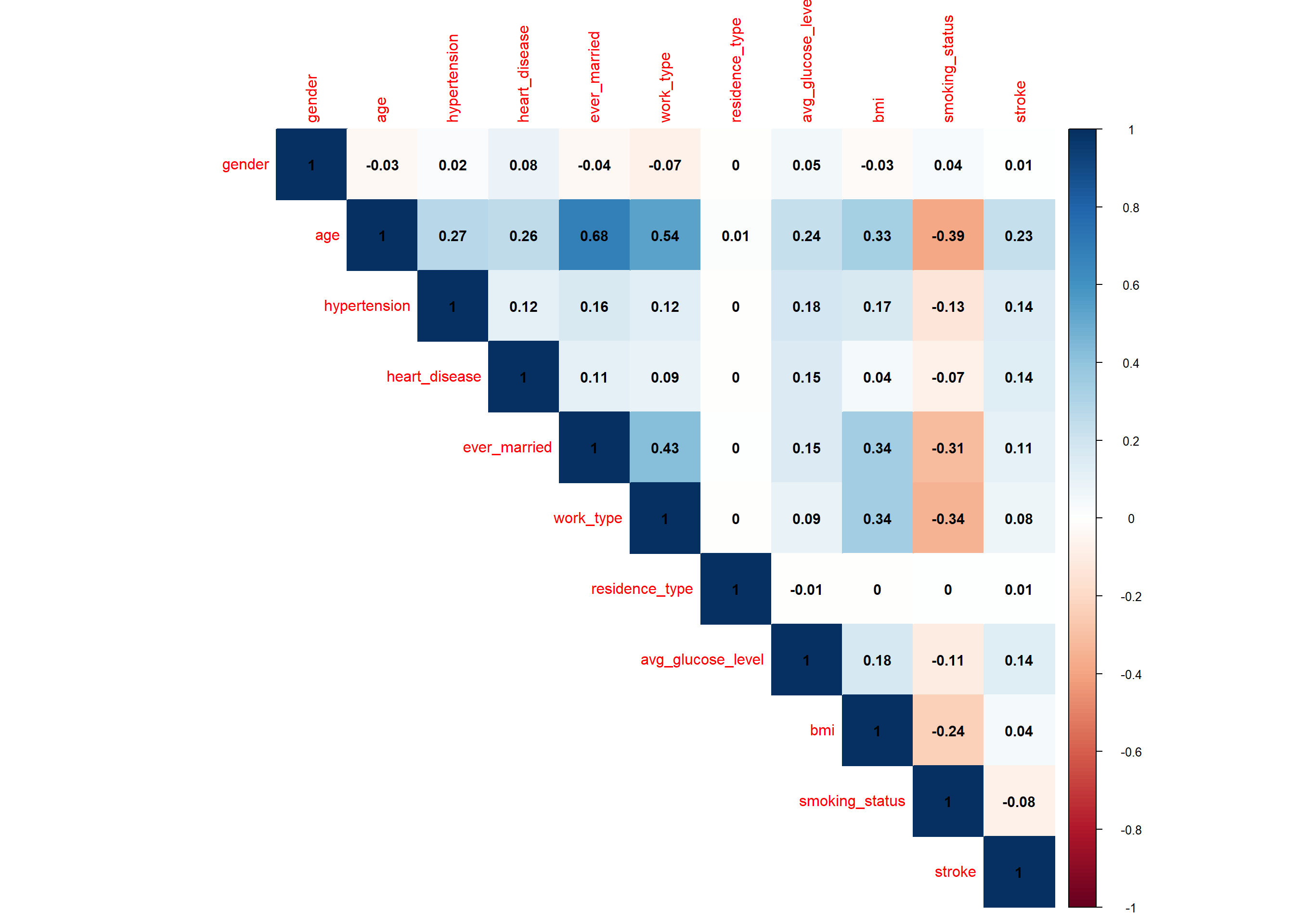
The variables gender, age, hypertension, heart disease, ever married, work type, residence type, average glucose level and bmi exhibit a positive linear association with our target variable (stroke) while smoking status a negative linear association.
# correlation tests for whole dataset
library(Hmisc)
res <- rcorr(as.matrix(stroke_final%>%
               dplyr::select(-id)%>%
         drop_na(bmi)%>%
               mutate(across(c(1:11), as.numeric)))) # rcorr() accepts matrices only

# display p-values (rounded to 3 decimals)
kable(
  round(res$P, 3)
)| gender | age | hypertension | heart_disease | ever_married | work_type | residence_type | avg_glucose_level | bmi | smoking_status | stroke | |
|---|---|---|---|---|---|---|---|---|---|---|---|
| gender | NA | 0.034 | 0.127 | 0.000 | 0.011 | 0.000 | 0.761 | 0.000 | 0.067 | 0.006 | 0.629 |
| age | 0.034 | NA | 0.000 | 0.000 | 0.000 | 0.000 | 0.450 | 0.000 | 0.000 | 0.000 | 0.000 |
| hypertension | 0.127 | 0.000 | NA | 0.000 | 0.000 | 0.000 | 0.936 | 0.000 | 0.000 | 0.000 | 0.000 |
| heart_disease | 0.000 | 0.000 | 0.000 | NA | 0.000 | 0.000 | 0.866 | 0.000 | 0.004 | 0.000 | 0.000 |
| ever_married | 0.011 | 0.000 | 0.000 | 0.000 | NA | 0.000 | 0.742 | 0.000 | 0.000 | 0.000 | 0.000 |
| work_type | 0.000 | 0.000 | 0.000 | 0.000 | 0.000 | NA | 0.955 | 0.000 | 0.000 | 0.000 | 0.000 |
| residence_type | 0.761 | 0.450 | 0.936 | 0.866 | 0.742 | 0.955 | NA | 0.602 | 0.984 | 0.865 | 0.675 |
| avg_glucose_level | 0.000 | 0.000 | 0.000 | 0.000 | 0.000 | 0.000 | 0.602 | NA | 0.000 | 0.000 | 0.000 |
| bmi | 0.067 | 0.000 | 0.000 | 0.004 | 0.000 | 0.000 | 0.984 | 0.000 | NA | 0.000 | 0.003 |
| smoking_status | 0.006 | 0.000 | 0.000 | 0.000 | 0.000 | 0.000 | 0.865 | 0.000 | 0.000 | NA | 0.000 |
| stroke | 0.629 | 0.000 | 0.000 | 0.000 | 0.000 | 0.000 | 0.675 | 0.000 | 0.003 | 0.000 | NA |
The linear association of stroke with gender and residence type is not significant (p>0.05).
3.2.2 Difference Frequency table
# make dataset with variables to summarize

tbl_summary(stroke_final%>%
               dplyr::select(-id),
              by = stroke,
                       type = list(
                         all_dichotomous() ~ "categorical",
                          all_continuous() ~ "continuous2")
                       , statistic = all_continuous() ~ c(
                                      "{mean} ({sd})",
                                      "{median} ({p25}, {p75})",
                                      "{min}, {max}")
                       , digits = all_continuous() ~ 2
                       , missing = "always" # don't list missing data separately
                       ,missing_text = "Missing"
                       ) %>%
   modify_header(label = "**Variables**") %>% # update the column header
   bold_labels() %>%
   italicize_levels()%>%
   add_n()%>% # add column with total number of non-missing observations
   add_p(pvalue_fun = ~style_pvalue(.x, digits = 3),
         test.args = c(work_type) ~ list(simulate.p.value=TRUE)) %>%
   bold_p(t= 0.05) %>% # bold p-values under a given threshold (default 0.05)
   #add_overall() %>%
   #add_difference() %>% #add column for difference between two group, confidence interval, and p-value
   modify_spanning_header(c("stat_1", "stat_2") ~ "**Stroke**")  %>%
   #modify_caption("**Table 1. Patient Characteristics**")%>%
   modify_footnote(
     all_stat_cols() ~ "Mean (SD); Median (IQR); Range; Frequency (%)"
)| Variables | N | Stroke | p-value2 | |
|---|---|---|---|---|
| No, N = 4,8601 | Yes, N = 2491 | |||
| Sex of the patient | 5,109 | 0.516 | ||
| Female | 2,853 (58.7%) | 141 (56.6%) | ||
| Male | 2,007 (41.3%) | 108 (43.4%) | ||
| Missing | 0 | 0 | ||
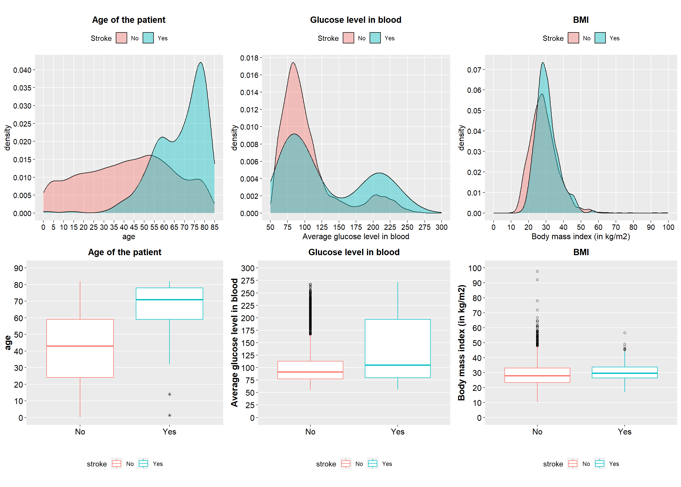
| Age of the patient | 5,109 | <0.001 | ||
| Mean (SD) | 41.97 (22.29) | 67.73 (12.73) | ||
| Median (IQR) | 43.00 (24.00, 59.00) | 71.00 (59.00, 78.00) | ||
| Range | 0.08, 82.00 | 1.32, 82.00 | ||
| Missing | 0 | 0 | ||
| Patient has hypertension | 5,109 | <0.001 | ||
| No | 4,428 (91.1%) | 183 (73.5%) | ||
| Yes | 432 (8.89%) | 66 (26.5%) | ||
| Missing | 0 | 0 | ||
| Patient has heart disease | 5,109 | <0.001 | ||
| No | 4,631 (95.3%) | 202 (81.1%) | ||
| Yes | 229 (4.71%) | 47 (18.9%) | ||
| Missing | 0 | 0 | ||
| Patient is married | 5,109 | <0.001 | ||
| No | 1,727 (35.5%) | 29 (11.6%) | ||
| Yes | 3,133 (64.5%) | 220 (88.4%) | ||
| Missing | 0 | 0 | ||
| Work type | 5,109 | <0.001 | ||
| children | 685 (14.1%) | 2 (0.80%) | ||
| Govt_job | 624 (12.8%) | 33 (13.3%) | ||
| Never_worked | 22 (0.45%) | 0 (0%) | ||
| Private | 2,775 (57.1%) | 149 (59.8%) | ||
| Self-employed | 754 (15.5%) | 65 (26.1%) | ||
| Missing | 0 | 0 | ||
| Residence type | 5,109 | 0.271 | ||
| Rural | 2,399 (49.4%) | 114 (45.8%) | ||
| Urban | 2,461 (50.6%) | 135 (54.2%) | ||
| Missing | 0 | 0 | ||
| Average glucose level in blood | 5,109 | <0.001 | ||
| Mean (SD) | 104.79 (43.85) | 132.54 (61.92) | ||
| Median (IQR) | 91.47 (77.12, 112.80) | 105.22 (79.79, 196.71) | ||
| Range | 55.12, 267.76 | 56.11, 271.74 | ||
| Missing | 0 | 0 | ||
| Body mass index (in kg/m2) | 4,908 | <0.001 | ||
| Mean (SD) | 28.82 (7.91) | 30.47 (6.33) | ||
| Median (IQR) | 28.00 (23.40, 33.10) | 29.70 (26.40, 33.70) | ||
| Range | 10.30, 97.60 | 16.90, 56.60 | ||
| Missing | 161 | 40 | ||
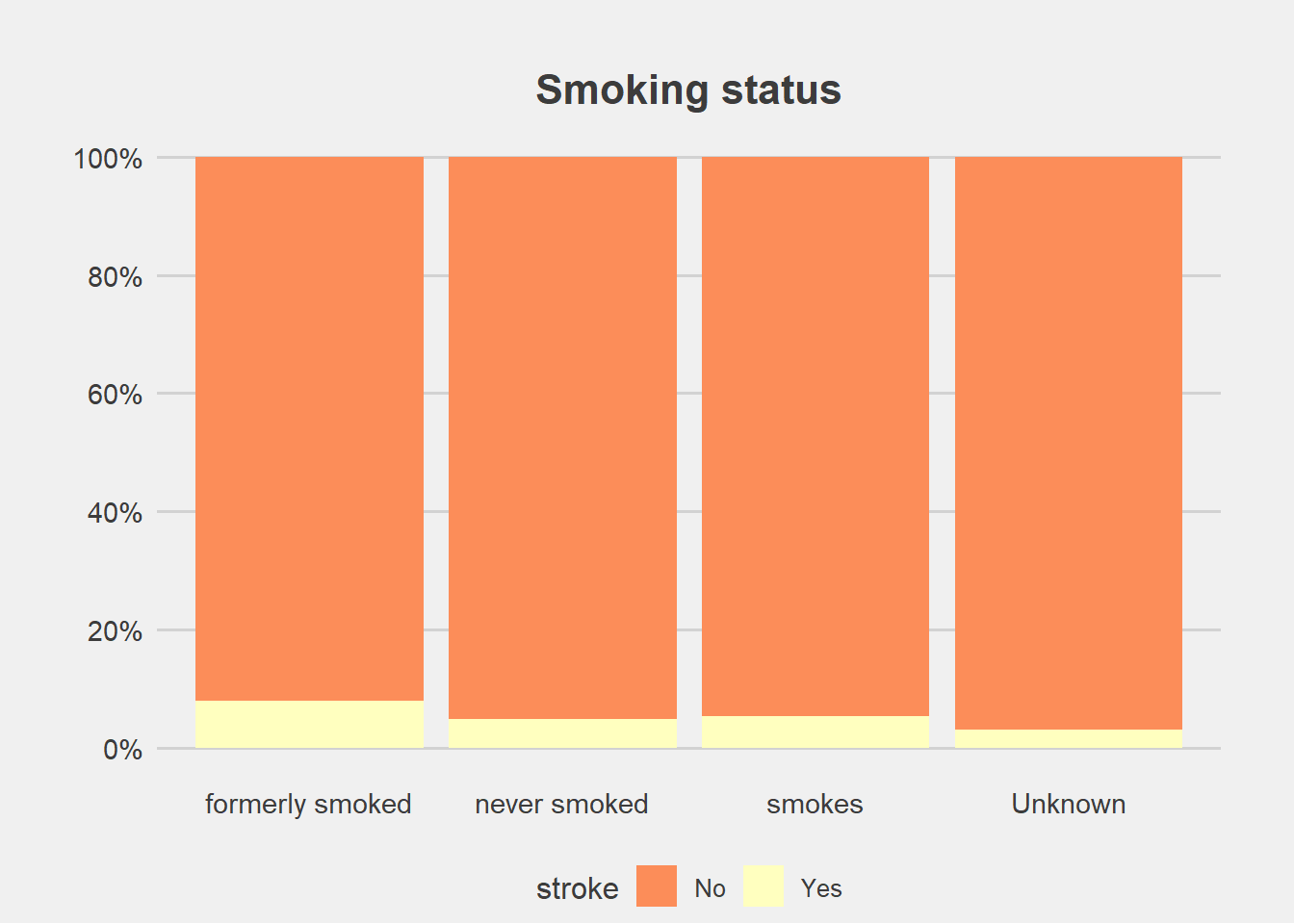
| Smoking status | 5,109 | <0.001 | ||
| formerly smoked | 814 (16.7%) | 70 (28.1%) | ||
| never smoked | 1,802 (37.1%) | 90 (36.1%) | ||
| smokes | 747 (15.4%) | 42 (16.9%) | ||
| Unknown | 1,497 (30.8%) | 47 (18.9%) | ||
| Missing | 0 | 0 | ||
| 1 Mean (SD); Median (IQR); Range; Frequency (%) | ||||
| 2 Pearson's Chi-squared test; Wilcoxon rank sum test; Fisher's Exact Test for Count Data with simulated p-value (based on 2000 replicates) | ||||
3.2.3 Visualization
library(ggthemes)

  ggplot(stroke_final, aes(x=gender))+
  geom_bar(aes(fill=stroke), position = "fill")+
  labs(title="Sex of the patient", y="Percent", x="")+
  scale_fill_brewer(palette = "Set1")+
  scale_y_continuous(breaks=seq(0,1,by=.2),label=scales::percent)+
  theme_fivethirtyeight()+
  theme(axis.title.y = element_blank(),
        #legend.title = element_blank(),
        plot.margin = unit(c(1,1,0,1),"cm"),
        axis.text = element_text(size = 11),
        plot.title = element_text(size=16,hjust = 0.5),
         panel.grid.major.x = element_blank())


  ggplot(stroke_final, aes(x=hypertension))+
  geom_bar(aes(fill=stroke), position = "fill")+
  labs(title="Patient has hypertension", y="Percent", x="")+
  scale_fill_brewer(palette = "Set2")+
  scale_y_continuous(breaks=seq(0,1,by=.2),label=scales::percent)+
  theme_fivethirtyeight()+
  theme(axis.title.y = element_blank(),
        #legend.title = element_blank(),
        plot.margin = unit(c(1,1,0,1),"cm"),
        axis.text = element_text(size = 11),
        plot.title = element_text(size=16,hjust = 0.5),
         panel.grid.major.x = element_blank())


  ggplot(stroke_final, aes(x=heart_disease))+
  geom_bar(aes(fill=stroke), position = "fill")+
  labs(title="Patient has heart disease", y="Percent", x="")+
  scale_fill_brewer(palette = "Set3")+
  scale_y_continuous(breaks=seq(0,1,by=.2),label=scales::percent)+
  theme_fivethirtyeight()+
  theme(axis.title.y = element_blank(),
        #legend.title = element_blank(),
        plot.margin = unit(c(1,1,0,1),"cm"),
        axis.text = element_text(size = 11),
        plot.title = element_text(size=16,hjust = 0.5),
         panel.grid.major.x = element_blank())


  ggplot(stroke_final, aes(x=ever_married))+
  geom_bar(aes(fill=stroke), position = "fill")+
  labs(title="Patient is married", y="Percent", x="")+
  scale_fill_brewer(palette = "Accent")+
  scale_y_continuous(breaks=seq(0,1,by=.2),label=scales::percent)+
  theme_fivethirtyeight()+
  theme(axis.title.y = element_blank(),
        #legend.title = element_blank(),
        plot.margin = unit(c(1,1,0,1),"cm"),
        axis.text = element_text(size = 11),
        plot.title = element_text(size=16,hjust = 0.5),
         panel.grid.major.x = element_blank())


  ggplot(stroke_final, aes(x=work_type))+
  geom_bar(aes(fill=stroke), position = "fill")+
  labs(title="Work type", y="Percent", x="")+
  scale_fill_brewer(palette = "Dark2")+
  scale_y_continuous(breaks=seq(0,1,by=.2),label=scales::percent)+
  theme_fivethirtyeight()+
  theme(axis.title.y = element_blank(),
        #legend.title = element_blank(),
        plot.margin = unit(c(1,1,0,1),"cm"),
        axis.text = element_text(size = 11),
        plot.title = element_text(size=16,hjust = 0.5),
         panel.grid.major.x = element_blank())


  ggplot(stroke_final, aes(x=residence_type))+
  geom_bar(aes(fill=stroke), position = "fill")+
  labs(title="Residence type", y="Percent", x="")+
  scale_fill_brewer(palette = "Paired")+
  scale_y_continuous(breaks=seq(0,1,by=.2),label=scales::percent)+
  theme_fivethirtyeight()+
  theme(axis.title.y = element_blank(),
        #legend.title = element_blank(),
        plot.margin = unit(c(1,1,0,1),"cm"),
        axis.text = element_text(size = 11),
        plot.title = element_text(size=16,hjust = 0.5),
         panel.grid.major.x = element_blank())


  ggplot(stroke_final, aes(x=smoking_status))+
  geom_bar(aes(fill=stroke), position = "fill")+
  labs(title="Smoking status", y="Percent", x="")+
  scale_fill_brewer(palette = "Spectral")+
  scale_y_continuous(breaks=seq(0,1,by=.2),label=scales::percent)+
  theme_fivethirtyeight()+
  theme(axis.title.y = element_blank(),
        #legend.title = element_blank(),
        plot.margin = unit(c(1,1,0,1),"cm"),
        axis.text = element_text(size = 11),
        plot.title = element_text(size=16,hjust = 0.5),
         panel.grid.major.x = element_blank())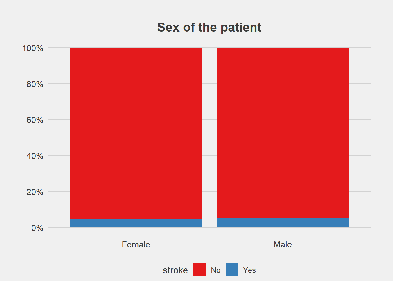
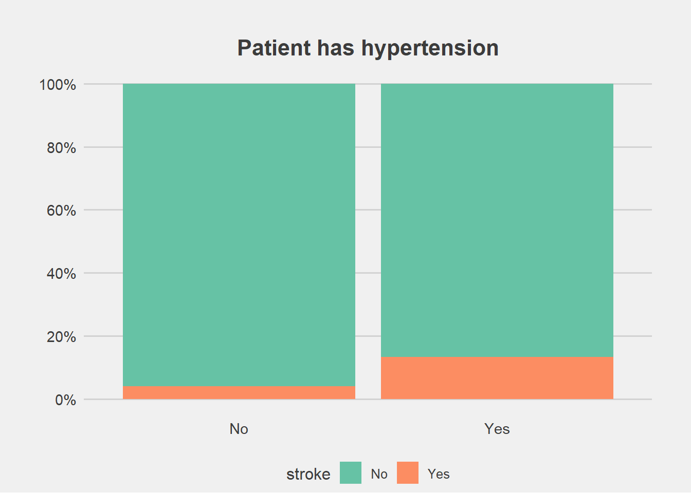
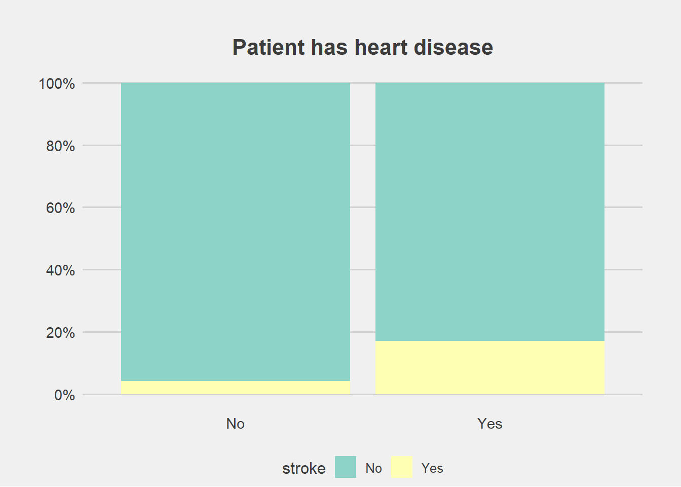
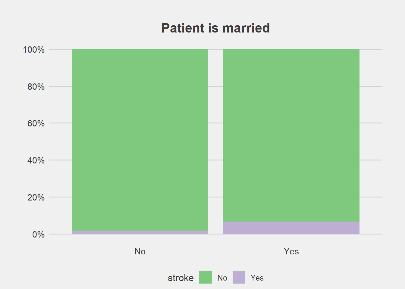
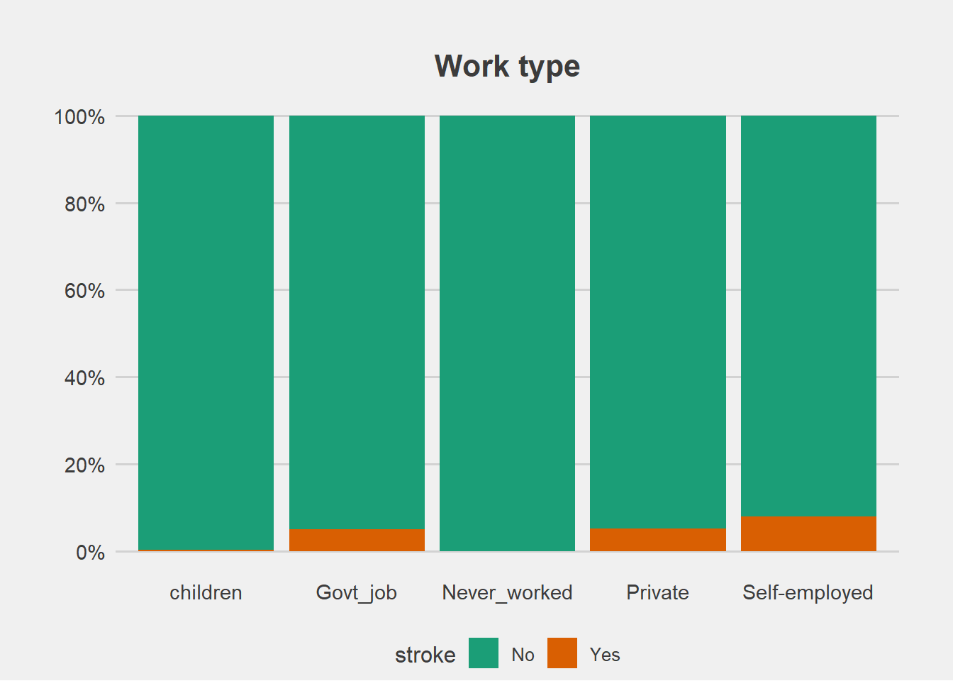
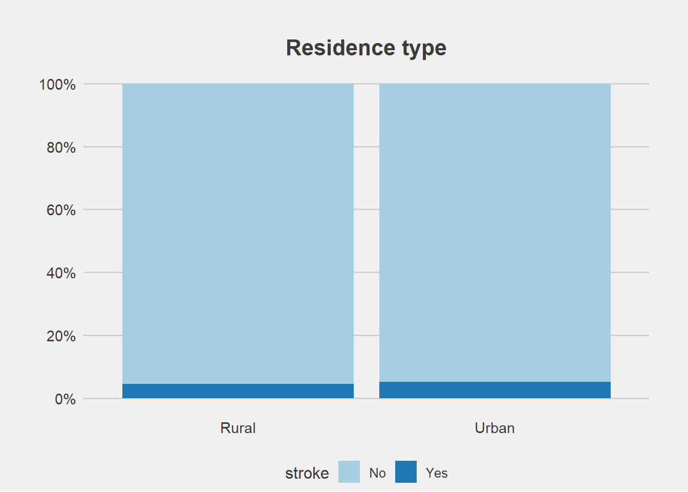
From the graphs, there is no difference in proportion of stroke with gender and residence type.
p1 <- ggplot(stroke_final, aes(x=age, fill=stroke)) +
  geom_density(alpha=0.4)+
  scale_y_continuous(n.breaks = 10)+
  scale_x_continuous(breaks = seq(0, 85, by = 5), limits = c(0, 85))+
  labs(x="age",y="density", title = "Age of the patient")+
  theme(axis.title = element_text(color="black",size=12),
        legend.position = "top",
        axis.text = element_text(color="black",size=11),
        plot.title = element_text(hjust = 0.5, face="bold",color="black",size=13),
        panel.grid.minor.y = element_blank(),
        panel.grid.minor.x = element_blank())+
  guides(fill = guide_legend(title = "Stroke"))


p2 <- ggplot(stroke_final, aes(x=avg_glucose_level, fill=stroke)) +
  geom_density(alpha=0.4)+
  scale_y_continuous(n.breaks = 10)+
  scale_x_continuous(breaks = seq(50, 300, by = 25), limits = c(50, 300))+
  labs(x="Average glucose level in blood",y="density", title = "Glucose level in blood")+
  theme(axis.title = element_text(color="black",size=12),
        legend.position = "top",
        axis.text = element_text(color="black",size=11),
        plot.title = element_text(hjust = 0.5, face="bold",color="black",size=13),
        panel.grid.minor.y = element_blank(),
        panel.grid.minor.x = element_blank())+
  guides(fill = guide_legend(title = "Stroke"))


p3 <- ggplot(stroke_final, aes(x=bmi, fill=stroke)) +
  geom_density(alpha=0.4)+
  scale_y_continuous(n.breaks = 10)+
  scale_x_continuous(breaks = seq(0, 100, by = 10), limits = c(0, 100))+
  labs(x="Body mass index (in kg/m2)",y="density", title = "BMI")+
  theme(axis.title = element_text(color="black",size=12),
        legend.position = "top",
        axis.text = element_text(color="black",size=11),
        plot.title = element_text(hjust = 0.5, face="bold",color="black",size=13),
        panel.grid.minor.y = element_blank(),
        panel.grid.minor.x = element_blank())+
  guides(fill = guide_legend(title = "Stroke"))


p4 <- ggplot(stroke_final, aes(stroke, age))+
  geom_boxplot(aes(colour = stroke), outlier.colour = "black",
               outlier.shape = 8, show.legend = TRUE)+
  labs(x="",y="age", title = "Age of the patient")+
  scale_y_continuous(breaks = seq(0, 90, by = 10), limits = c(0, 90))+
  theme(axis.title = element_text(face="bold",color="black",size=13),
        legend.position = "bottom",
        axis.text = element_text(color="black",size=12),
        plot.title = element_text(hjust = 0.5, face="bold",color="black",size=13),
        panel.grid.major.x = element_blank(),
        panel.grid.minor.y = element_blank())


p5 <- ggplot(stroke_final, aes(stroke, avg_glucose_level))+
  geom_boxplot(aes(colour = stroke), outlier.colour = "black",
               outlier.shape = 1, show.legend = TRUE)+
  labs(x="",y="Average glucose level in blood", title = "Glucose level in blood")+
  scale_y_continuous(breaks = seq(0, 300, by = 25), limits = c(0, 300))+
  theme(axis.title = element_text(face="bold",color="black",size=13),
        legend.position = "bottom",
        axis.text = element_text(color="black",size=12),
        plot.title = element_text(hjust = 0.5, face="bold",color="black",size=13),
        panel.grid.major.x = element_blank(),
        panel.grid.minor.y = element_blank())


p6 <- ggplot(stroke_final, aes(stroke, bmi))+
  geom_boxplot(aes(colour = stroke), outlier.colour = "black",
               outlier.shape = 1, show.legend = TRUE)+
  labs(x="",y="Body mass index (in kg/m2)", title = "BMI")+
  scale_y_continuous(breaks = seq(0, 100, by = 10), limits = c(0, 100))+
  theme(axis.title = element_text(face="bold",color="black",size=13),
        legend.position = "bottom",
        axis.text = element_text(color="black",size=12),
        plot.title = element_text(hjust = 0.5, face="bold",color="black",size=13),
        panel.grid.major.x = element_blank(),
        panel.grid.minor.y = element_blank())


figure1 <- ggarrange( p1, p2, p3, p4, p5, p6,
          ncol = 3, nrow = 2)

annotate_figure(figure1,
                top = text_grob("",
                                color = "red", face = "bold", size = 15),
                bottom = text_grob("", color = "blue",
                                   hjust = 1, x = 0.98, face = "italic", size = 10),
                #left = text_grob("Figure arranged using ggpubr", color = "green", rot = 90),
                #right = "",
                fig.lab = "", fig.lab.face = "bold"
                )
4 Modelling
From the exploration done, it is very hard to make a conclusion. The dependent variable “stroke” is imbalanced. Patient had stroke (4.9%) vs Patient who did no have stroke (95.1%). It will be very wrong to just perform a predictive model on such kind of data without making any changes.
Before creating any model, the first step is to drop missing cases and irrelevant variabled (id) then divide the data into training and testing dataset.
stroke_model <- stroke_final%>%
              dplyr::select(-id)%>%
  drop_na()

table(stroke_model$stroke)
##
## No Yes
## 4699 209library(caTools)
set.seed(123)
sample <- sample.split(stroke_model$stroke, SplitRatio = 0.8)
train <- subset(stroke_model, sample==TRUE)
test <- subset(stroke_model, sample==FALSE)
#train=stroke_model[sample==TRUE, ]
#test=stroke_model
table(train$stroke)##
## No Yes
## 3759 167table(test$stroke)##
## No Yes
## 940 424.1 Random Forest - categorical
4.1.1 Imbalanced Data
library(randomForest)

model1_rf <- randomForest(stroke ~., data = train)
model1_rf
##
## Call:
## randomForest(formula = stroke ~ ., data = train)
## Type of random forest: classification
## Number of trees: 500
## No. of variables tried at each split: 3
##
## OOB estimate of error rate: 4.28%
## Confusion matrix:
## No Yes class.error
## No 3758 1 0.0002660282
## Yes 167 0 1.0000000000library(caret)
confusionMatrix(predict(model1_rf, test), test$stroke, positive = "Yes")## Confusion Matrix and Statistics
##
## Reference
## Prediction No Yes
## No 940 42
## Yes 0 0
##
## Accuracy : 0.9572
## 95% CI : (0.9426, 0.969)
## No Information Rate : 0.9572
## P-Value [Acc > NIR] : 0.5409
##
## Kappa : 0
##
## Mcnemar's Test P-Value : 2.509e-10
##
## Sensitivity : 0.00000
## Specificity : 1.00000
## Pos Pred Value : NaN
## Neg Pred Value : 0.95723
## Prevalence : 0.04277
## Detection Rate : 0.00000
## Detection Prevalence : 0.00000
## Balanced Accuracy : 0.50000
##
## 'Positive' Class : Yes
## From the above output we can see that the accuracy of the model is 95.72%.
However we need to be sure that this model is good by checking the sensitivity and the specificity. Sensitivity is the accuracy of predicting what we are interested in, that is a person having experienced a stroke while specificity is now for no stroke.
From the output the sensitivity is at 0% while specificity is 100%. This means that this model will be more accurate in predicting those who did not have stroke than those who did. This problem has been caused by the imbalance of the dependent variable.
This problem can be solved in several ways including; over sampling, undersampling and both. We will use the package called ROSE.
library(ROSE)4.1.2 Oversampling data
We specify N=7518 (3759x2). Over sampling repeats some values in the category with the fewer entries randomly until they are the same with the larger entry.
over_sampling <-ovun.sample(stroke ~.,data=train, method = "over", N=7518, seed=1)$data

table(over_sampling$stroke)
##
## No Yes
## 3759 3759model2_rf <- randomForest(stroke ~., data = over_sampling)
model2_rf##
## Call:
## randomForest(formula = stroke ~ ., data = over_sampling)
## Type of random forest: classification
## Number of trees: 500
## No. of variables tried at each split: 3
##
## OOB estimate of error rate: 0.76%
## Confusion matrix:
## No Yes class.error
## No 3702 57 0.01516361
## Yes 0 3759 0.00000000confusionMatrix(predict(model2_rf, test), test$stroke, positive = "Yes")## Confusion Matrix and Statistics
##
## Reference
## Prediction No Yes
## No 932 41
## Yes 8 1
##
## Accuracy : 0.9501
## 95% CI : (0.9346, 0.9629)
## No Information Rate : 0.9572
## P-Value [Acc > NIR] : 0.88
##
## Kappa : 0.0245
##
## Mcnemar's Test P-Value : 4.844e-06
##
## Sensitivity : 0.023810
## Specificity : 0.991489
## Pos Pred Value : 0.111111
## Neg Pred Value : 0.957862
## Prevalence : 0.042770
## Detection Rate : 0.001018
## Detection Prevalence : 0.009165
## Balanced Accuracy : 0.507649
##
## 'Positive' Class : Yes
## From the output above, we can see that sensitivity is 2.38% while specificity has gone down to 99.15%. This proportion is not still good.
4.1.3 Under sampling data
This reduces the entries in the category with more entries to be the same with the one with few entries hence (167*2=334).
under_sampling <-ovun.sample(stroke ~.,data=train, method = "under", N=334, seed=2)$data

table(under_sampling$stroke)
##
## No Yes
## 167 167model3_rf <- randomForest(stroke ~., data = under_sampling)
model3_rf##
## Call:
## randomForest(formula = stroke ~ ., data = under_sampling)
## Type of random forest: classification
## Number of trees: 500
## No. of variables tried at each split: 3
##
## OOB estimate of error rate: 25.15%
## Confusion matrix:
## No Yes class.error
## No 114 53 0.3173653
## Yes 31 136 0.1856287confusionMatrix(predict(model3_rf, test), test$stroke, positive = "Yes")## Confusion Matrix and Statistics
##
## Reference
## Prediction No Yes
## No 680 10
## Yes 260 32
##
## Accuracy : 0.7251
## 95% CI : (0.696, 0.7528)
## No Information Rate : 0.9572
## P-Value [Acc > NIR] : 1
##
## Kappa : 0.1263
##
## Mcnemar's Test P-Value : <2e-16
##
## Sensitivity : 0.76190
## Specificity : 0.72340
## Pos Pred Value : 0.10959
## Neg Pred Value : 0.98551
## Prevalence : 0.04277
## Detection Rate : 0.03259
## Detection Prevalence : 0.29735
## Balanced Accuracy : 0.74265
##
## 'Positive' Class : Yes
## From the output above, sensitivity now stands at 76.19% while specificity stands at 72.34%. This is a better model than the unbalanced and over sampled model.
4.1.4 Both Sampling data
both_sampling <- ovun.sample(stroke~.,data=train, method="both",p=0.5, seed=222, N=3926)$data

table(both_sampling$stroke)
##
## No Yes
## 1947 1979model4_rf <- randomForest(stroke ~., data = both_sampling)
model4_rf##
## Call:
## randomForest(formula = stroke ~ ., data = both_sampling)
## Type of random forest: classification
## Number of trees: 500
## No. of variables tried at each split: 3
##
## OOB estimate of error rate: 1.32%
## Confusion matrix:
## No Yes class.error
## No 1895 52 0.02670776
## Yes 0 1979 0.00000000confusionMatrix(predict(model4_rf, test), test$stroke, positive = "Yes")## Confusion Matrix and Statistics
##
## Reference
## Prediction No Yes
## No 911 31
## Yes 29 11
##
## Accuracy : 0.9389
## 95% CI : (0.922, 0.9531)
## No Information Rate : 0.9572
## P-Value [Acc > NIR] : 0.9972
##
## Kappa : 0.2364
##
## Mcnemar's Test P-Value : 0.8973
##
## Sensitivity : 0.26190
## Specificity : 0.96915
## Pos Pred Value : 0.27500
## Neg Pred Value : 0.96709
## Prevalence : 0.04277
## Detection Rate : 0.01120
## Detection Prevalence : 0.04073
## Balanced Accuracy : 0.61553
##
## 'Positive' Class : Yes
## From the output above, the sensitivity now is at 26.19% while specificity is at 96.92%.
- This means that the under sampled random forest model is the best to predict stroke with test accuracy of 72.51%, sensitivity of 76.19% and specificity of 72.34%.
4.2 Tree
library(tree)4.2.1 Unpruned classification tree
4.2.1.1 Imbalanced data - all data
stroke_tree = tree(stroke ~ ., data = stroke_model)

#stroke_tree = tree(stroke ~ ., data = stroke_model, control = tree.control(nobs = nrow(stroke_model), minsize = 10))

summary(stroke_tree)
##
## Classification tree:
## tree(formula = stroke ~ ., data = stroke_model)
## Variables actually used in tree construction:
## [1] "age"
## Number of terminal nodes: 4
## Residual mean deviance: 0.2853 = 1399 / 4904
## Misclassification error rate: 0.04258 = 209 / 4908stroke_tree## node), split, n, deviance, yval, (yprob)
## * denotes terminal node
##
## 1) root 4908 1728.00 No ( 0.957416 0.042584 )
## 2) age < 53.5 3150 320.20 No ( 0.991111 0.008889 )
## 4) age < 37.5 1974 31.58 No ( 0.998987 0.001013 ) *
## 5) age > 37.5 1176 249.60 No ( 0.977891 0.022109 ) *
## 3) age > 53.5 1758 1166.00 No ( 0.897042 0.102958 )
## 6) age < 67.5 967 427.80 No ( 0.942089 0.057911 ) *
## 7) age > 67.5 791 690.40 No ( 0.841972 0.158028 ) *plot(stroke_tree)
text(stroke_tree, pretty = 0)
title(main = "Unpruned Classification Tree - All data")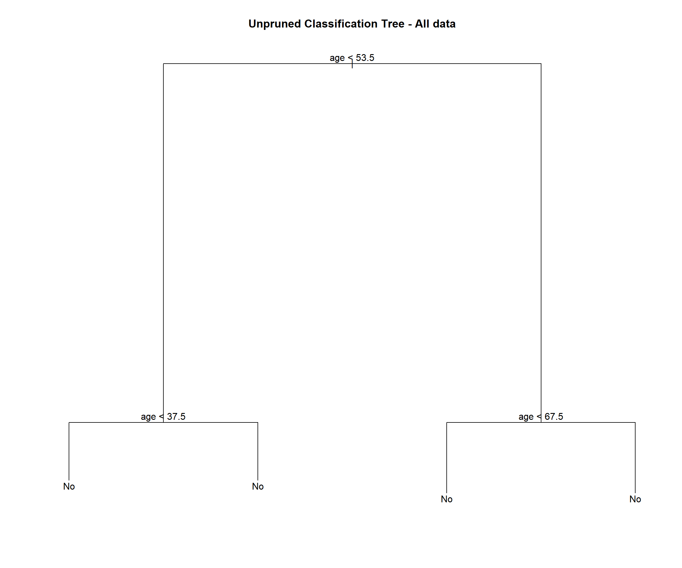
summary(stroke_tree)$used## [1] age
## 11 Levels: <leaf> gender age hypertension heart_disease ... smoking_statusnames(stroke_model)[which(!(names(stroke_model) %in% summary(stroke_tree)$used))]## [1] "gender" "hypertension" "heart_disease"
## [4] "ever_married" "work_type" "residence_type"
## [7] "avg_glucose_level" "bmi" "smoking_status"
## [10] "stroke"We see this tree has 4 terminal nodes and a misclassification rate of 0.04258. The tree is not using all of the available variables. It has only used 1 variable (age).
4.2.1.2 Imbalanced data - train
stroke_tree_train = tree(stroke ~ ., data = train)


summary(stroke_tree_train)
##
## Classification tree:
## tree(formula = stroke ~ ., data = train)
## Variables actually used in tree construction:
## [1] "age" "smoking_status" "avg_glucose_level"
## Number of terminal nodes: 6
## Residual mean deviance: 0.2789 = 1093 / 3920
## Misclassification error rate: 0.04254 = 167 / 3926stroke_tree_train## node), split, n, deviance, yval, (yprob)
## * denotes terminal node
##
## 1) root 3926 1381.00 No ( 0.957463 0.042537 )
## 2) age < 56.5 2692 329.50 No ( 0.988856 0.011144 )
## 4) age < 37.5 1569 30.66 No ( 0.998725 0.001275 ) *
## 5) age > 37.5 1123 262.00 No ( 0.975067 0.024933 ) *
## 3) age > 56.5 1234 860.50 No ( 0.888979 0.111021 )
## 6) age < 67.5 587 281.50 No ( 0.935264 0.064736 )
## 12) smoking_status: never smoked,Unknown 323 82.19 No ( 0.972136 0.027864 ) *
## 13) smoking_status: formerly smoked,smokes 264 182.80 No ( 0.890152 0.109848 )
## 26) avg_glucose_level < 106.955 169 64.42 No ( 0.952663 0.047337 ) *
## 27) avg_glucose_level > 106.955 95 100.40 No ( 0.778947 0.221053 ) *
## 7) age > 67.5 647 553.70 No ( 0.846986 0.153014 ) *plot(stroke_tree_train)
text(stroke_tree_train, pretty = 1)
title(main = "Unpruned Classification Tree - Train data")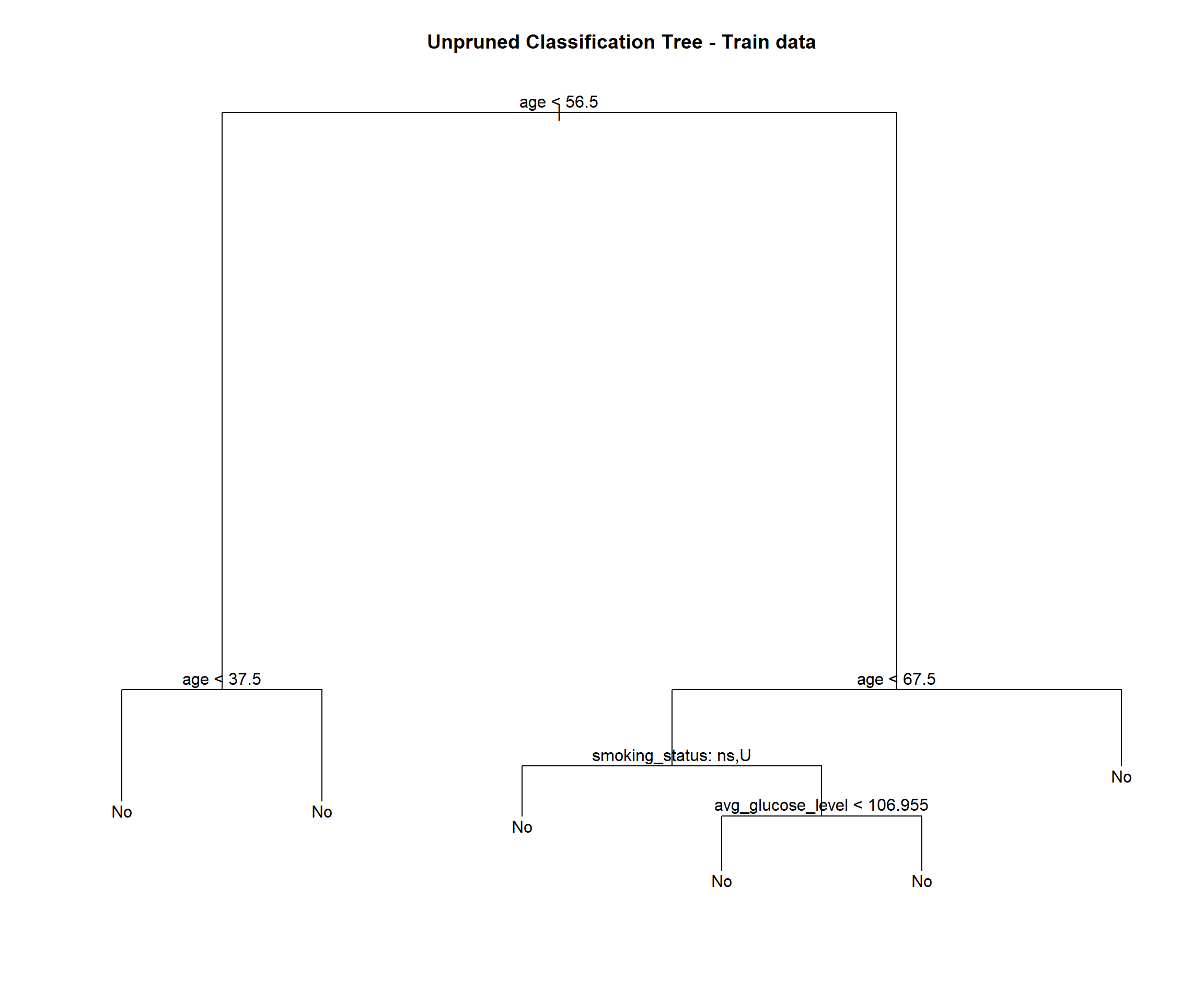
summary(stroke_tree_train)$used## [1] age smoking_status avg_glucose_level
## 11 Levels: <leaf> gender age hypertension heart_disease ... smoking_statusnames(train)[which(!(names(train) %in% summary(stroke_tree_train)$used))]## [1] "gender" "hypertension" "heart_disease" "ever_married"
## [5] "work_type" "residence_type" "bmi" "stroke"This tree is slightly different than the tree fit to all of the data.
We see this tree has 6 terminal nodes and a misclassification rate of 0.04254. The tree is not using all of the available variables. It has only used 3 variables( age, smoking status and average glucose level).
When using the predict() function on a tree, the default type is vector which gives predicted probabilities for both classes. We will use type = class to directly obtain classes.
confusionMatrix(predict(stroke_tree_train, train, type = "class"), train$stroke, positive = "Yes")## Confusion Matrix and Statistics
##
## Reference
## Prediction No Yes
## No 3759 167
## Yes 0 0
##
## Accuracy : 0.9575
## 95% CI : (0.9507, 0.9636)
## No Information Rate : 0.9575
## P-Value [Acc > NIR] : 0.5206
##
## Kappa : 0
##
## Mcnemar's Test P-Value : <2e-16
##
## Sensitivity : 0.00000
## Specificity : 1.00000
## Pos Pred Value : NaN
## Neg Pred Value : 0.95746
## Prevalence : 0.04254
## Detection Rate : 0.00000
## Detection Prevalence : 0.00000
## Balanced Accuracy : 0.50000
##
## 'Positive' Class : Yes
## confusionMatrix(predict(stroke_tree_train, test, type = "class"), test$stroke, positive = "Yes")## Confusion Matrix and Statistics
##
## Reference
## Prediction No Yes
## No 940 42
## Yes 0 0
##
## Accuracy : 0.9572
## 95% CI : (0.9426, 0.969)
## No Information Rate : 0.9572
## P-Value [Acc > NIR] : 0.5409
##
## Kappa : 0
##
## Mcnemar's Test P-Value : 2.509e-10
##
## Sensitivity : 0.00000
## Specificity : 1.00000
## Pos Pred Value : NaN
## Neg Pred Value : 0.95723
## Prevalence : 0.04277
## Detection Rate : 0.00000
## Detection Prevalence : 0.00000
## Balanced Accuracy : 0.50000
##
## 'Positive' Class : Yes
## Here it is easy to see that the tree is not a good fit. From both outputs the sensitivity is at 0% while specificity is 100%. This means that this model will be more accurate in predicting those who did not have stroke than those who did. This problem has been caused by the imbalance of the dependent variable.
4.2.1.3 Oversampling data
stroke_tree_over = tree(stroke ~ ., data = over_sampling)


summary(stroke_tree_over)
##
## Classification tree:
## tree(formula = stroke ~ ., data = over_sampling)
## Variables actually used in tree construction:
## [1] "age" "avg_glucose_level" "smoking_status"
## [4] "bmi"
## Number of terminal nodes: 9
## Residual mean deviance: 0.877 = 6585 / 7509
## Misclassification error rate: 0.2264 = 1702 / 7518stroke_tree_over## node), split, n, deviance, yval, (yprob)
## * denotes terminal node
##
## 1) root 7518 10420.00 No ( 0.50000 0.50000 )
## 2) age < 44.5 2101 1131.00 No ( 0.92385 0.07615 )
## 4) avg_glucose_level < 83.415 916 848.60 No ( 0.82533 0.17467 )
## 8) avg_glucose_level < 83.2 853 632.50 No ( 0.87808 0.12192 )
## 16) smoking_status: never smoked,Unknown 611 215.00 No ( 0.95745 0.04255 )
## 32) avg_glucose_level < 57.935 64 86.46 No ( 0.59375 0.40625 ) *
## 33) avg_glucose_level > 57.935 547 0.00 No ( 1.00000 0.00000 ) *
## 17) smoking_status: formerly smoked,smokes 242 304.20 No ( 0.67769 0.32231 ) *
## 9) avg_glucose_level > 83.2 63 43.95 Yes ( 0.11111 0.88889 ) *
## 5) avg_glucose_level > 83.415 1185 0.00 No ( 1.00000 0.00000 ) *
## 3) age > 44.5 5417 6913.00 Yes ( 0.33561 0.66439 )
## 6) age < 67.5 2642 3659.00 Yes ( 0.48070 0.51930 )
## 12) bmi < 27.25 507 597.50 No ( 0.72387 0.27613 )
## 24) smoking_status: formerly smoked,Unknown 144 0.00 No ( 1.00000 0.00000 ) *
## 25) smoking_status: never smoked,smokes 363 484.10 No ( 0.61433 0.38567 ) *
## 13) bmi > 27.25 2135 2909.00 Yes ( 0.42295 0.57705 ) *
## 7) age > 67.5 2775 2758.00 Yes ( 0.19748 0.80252 ) *plot(stroke_tree_over)
text(stroke_tree_over, pretty = 1)
title(main = "Unpruned Classification Tree - over sampling data")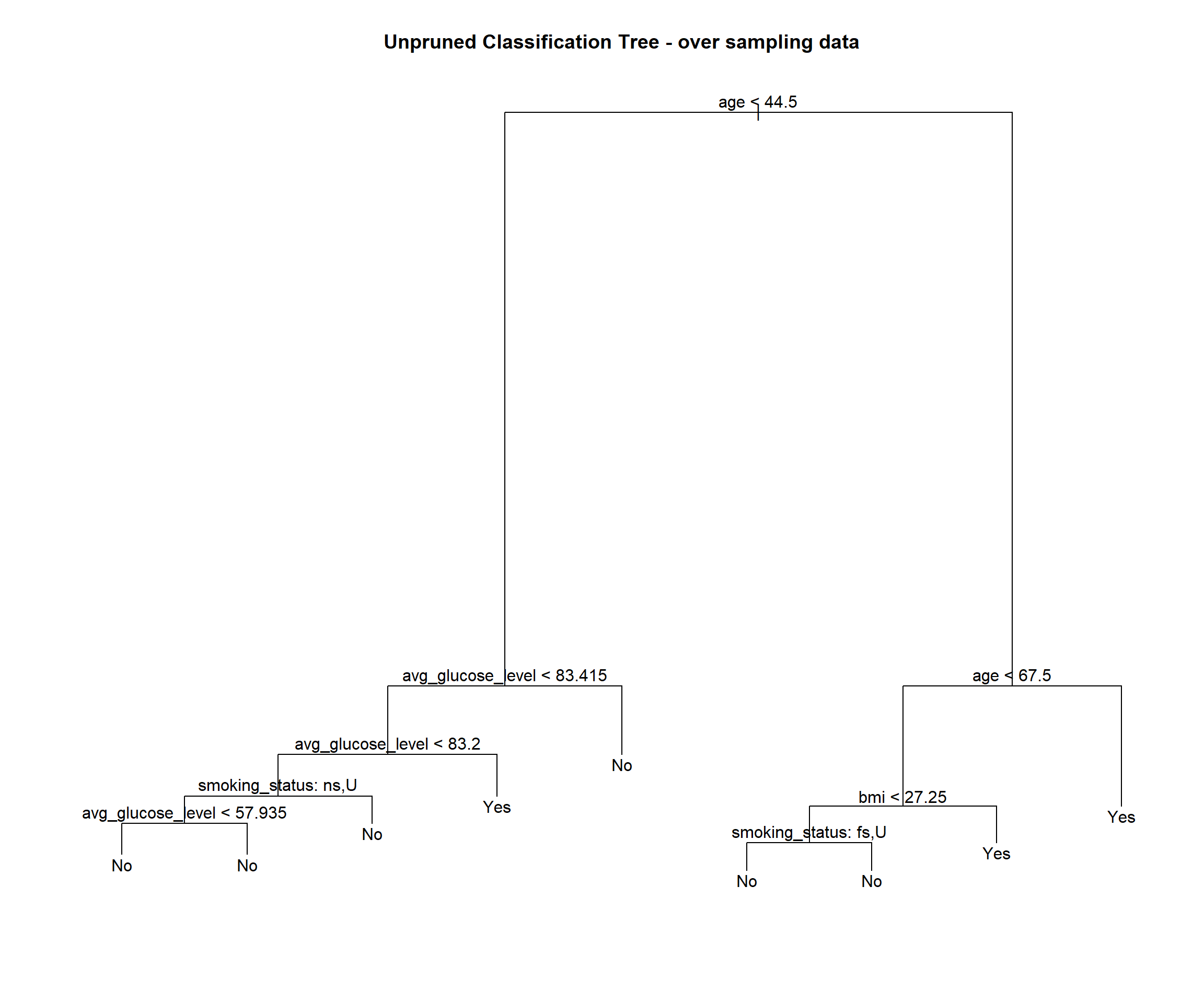
summary(stroke_tree_over)$used## [1] age avg_glucose_level smoking_status bmi
## 11 Levels: <leaf> gender age hypertension heart_disease ... smoking_statusnames(over_sampling)[which(!(names(over_sampling) %in% summary(stroke_tree_over)$used))]## [1] "gender" "hypertension" "heart_disease" "ever_married"
## [5] "work_type" "residence_type" "stroke"We see this tree has 9 terminal nodes and a misclassification rate of 0.2264. The tree has only used 4 vaiables (age, smoking status, average glucose level and bmi).
confusionMatrix(predict(stroke_tree_over, over_sampling, type = "class"), over_sampling$stroke, positive = "Yes")## Confusion Matrix and Statistics
##
## Reference
## Prediction No Yes
## No 2301 244
## Yes 1458 3515
##
## Accuracy : 0.7736
## 95% CI : (0.764, 0.783)
## No Information Rate : 0.5
## P-Value [Acc > NIR] : < 2.2e-16
##
## Kappa : 0.5472
##
## Mcnemar's Test P-Value : < 2.2e-16
##
## Sensitivity : 0.9351
## Specificity : 0.6121
## Pos Pred Value : 0.7068
## Neg Pred Value : 0.9041
## Prevalence : 0.5000
## Detection Rate : 0.4675
## Detection Prevalence : 0.6615
## Balanced Accuracy : 0.7736
##
## 'Positive' Class : Yes
## confusionMatrix(predict(stroke_tree_over, test, type = "class"), test$stroke, positive = "Yes")## Confusion Matrix and Statistics
##
## Reference
## Prediction No Yes
## No 595 4
## Yes 345 38
##
## Accuracy : 0.6446
## 95% CI : (0.6138, 0.6746)
## No Information Rate : 0.9572
## P-Value [Acc > NIR] : 1
##
## Kappa : 0.1102
##
## Mcnemar's Test P-Value : <2e-16
##
## Sensitivity : 0.90476
## Specificity : 0.63298
## Pos Pred Value : 0.09922
## Neg Pred Value : 0.99332
## Prevalence : 0.04277
## Detection Rate : 0.03870
## Detection Prevalence : 0.39002
## Balanced Accuracy : 0.76887
##
## 'Positive' Class : Yes
## Here it is easy to see that the tree is a better fit than the unbalanced train model. From both outputs the sensitivity has increased to the 90% range while specificity has decreased to 60% range.
However the tree has been over-fit. The over sampling train set performs much better than the test set.
Overfitting happens when a model learns the detail and noise in the training data to the extent that it negatively impacts the performance of the model on new data. This means that the noise or random fluctuations in the training data is picked up and learned as concepts by the model.
4.2.1.4 Under sampling data
stroke_tree_under = tree(stroke ~ ., data = under_sampling)


summary(stroke_tree_under)
##
## Classification tree:
## tree(formula = stroke ~ ., data = under_sampling)
## Variables actually used in tree construction:
## [1] "age" "avg_glucose_level" "smoking_status"
## [4] "hypertension"
## Number of terminal nodes: 9
## Residual mean deviance: 0.8516 = 276.8 / 325
## Misclassification error rate: 0.1946 = 65 / 334stroke_tree_under## node), split, n, deviance, yval, (yprob)
## * denotes terminal node
##
## 1) root 334 463.000 No ( 0.50000 0.50000 )
## 2) age < 44.5 95 44.760 No ( 0.93684 0.06316 )
## 4) avg_glucose_level < 83.425 39 33.490 No ( 0.84615 0.15385 )
## 8) avg_glucose_level < 80.005 34 20.290 No ( 0.91176 0.08824 )
## 16) smoking_status: formerly smoked,never smoked,Unknown 29 8.700 No ( 0.96552 0.03448 ) *
## 17) smoking_status: smokes 5 6.730 No ( 0.60000 0.40000 ) *
## 9) avg_glucose_level > 80.005 5 6.730 Yes ( 0.40000 0.60000 ) *
## 5) avg_glucose_level > 83.425 56 0.000 No ( 1.00000 0.00000 ) *
## 3) age > 44.5 239 301.900 Yes ( 0.32636 0.67364 )
## 6) age < 67.5 119 164.800 Yes ( 0.47899 0.52101 )
## 12) smoking_status: never smoked,Unknown 61 81.770 No ( 0.60656 0.39344 )
## 24) hypertension: No 52 65.730 No ( 0.67308 0.32692 ) *
## 25) hypertension: Yes 9 9.535 Yes ( 0.22222 0.77778 ) *
## 13) smoking_status: formerly smoked,smokes 58 74.730 Yes ( 0.34483 0.65517 ) *
## 7) age > 67.5 120 111.300 Yes ( 0.17500 0.82500 )
## 14) age < 70.5 16 0.000 Yes ( 0.00000 1.00000 ) *
## 15) age > 70.5 104 104.600 Yes ( 0.20192 0.79808 ) *plot(stroke_tree_under)
text(stroke_tree_under, pretty = 1)
title(main = "Unpruned Classification Tree - under sampling data")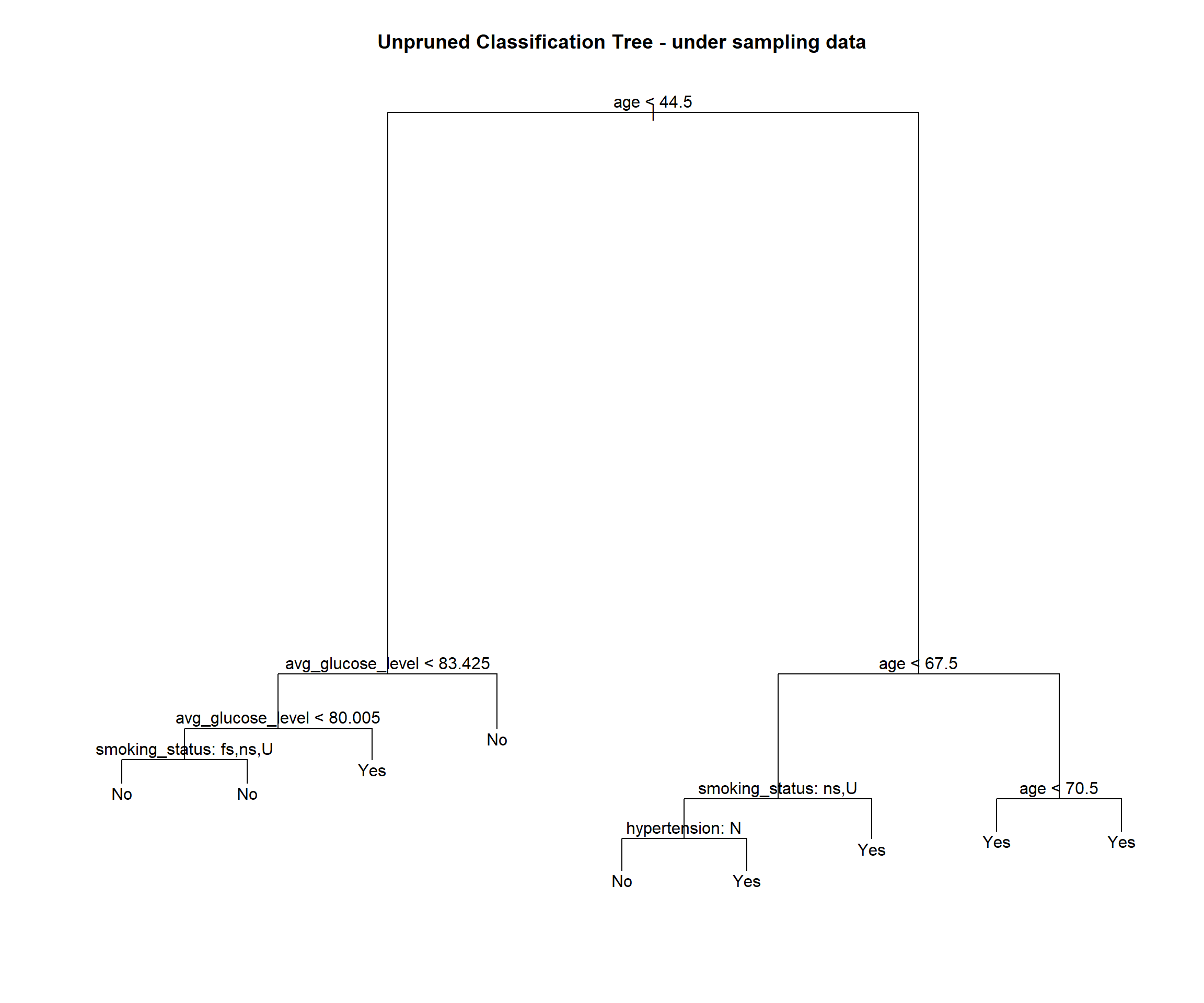
summary(stroke_tree_under)$used## [1] age avg_glucose_level smoking_status hypertension
## 11 Levels: <leaf> gender age hypertension heart_disease ... smoking_statusnames(under_sampling)[which(!(names(under_sampling) %in% summary(stroke_tree_under)$used))]## [1] "gender" "heart_disease" "ever_married" "work_type"
## [5] "residence_type" "bmi" "stroke"We see this tree has 9 terminal nodes and a misclassification rate of 0.1946. The tree has only used 4 vaiables (age, smoking status, average glucose level and hypertension).
confusionMatrix(predict(stroke_tree_under, under_sampling, type = "class"), under_sampling$stroke, positive = "Yes")## Confusion Matrix and Statistics
##
## Reference
## Prediction No Yes
## No 122 20
## Yes 45 147
##
## Accuracy : 0.8054
## 95% CI : (0.7588, 0.8465)
## No Information Rate : 0.5
## P-Value [Acc > NIR] : < 2.2e-16
##
## Kappa : 0.6108
##
## Mcnemar's Test P-Value : 0.002912
##
## Sensitivity : 0.8802
## Specificity : 0.7305
## Pos Pred Value : 0.7656
## Neg Pred Value : 0.8592
## Prevalence : 0.5000
## Detection Rate : 0.4401
## Detection Prevalence : 0.5749
## Balanced Accuracy : 0.8054
##
## 'Positive' Class : Yes
## confusionMatrix(predict(stroke_tree_under, test, type = "class"), test$stroke, positive = "Yes")## Confusion Matrix and Statistics
##
## Reference
## Prediction No Yes
## No 622 8
## Yes 318 34
##
## Accuracy : 0.668
## 95% CI : (0.6376, 0.6974)
## No Information Rate : 0.9572
## P-Value [Acc > NIR] : 1
##
## Kappa : 0.1041
##
## Mcnemar's Test P-Value : <2e-16
##
## Sensitivity : 0.80952
## Specificity : 0.66170
## Pos Pred Value : 0.09659
## Neg Pred Value : 0.98730
## Prevalence : 0.04277
## Detection Rate : 0.03462
## Detection Prevalence : 0.35845
## Balanced Accuracy : 0.73561
##
## 'Positive' Class : Yes
## Here it is easy to see that the tree is a better fit than the unbalanced train model and over sampled train model (less accuracy).
However the tree has been over-fit. The under sampling train set performs much better than the test set.
4.2.1.5 Both sampling data
stroke_tree_both = tree(stroke ~ ., data = both_sampling)


summary(stroke_tree_both)
##
## Classification tree:
## tree(formula = stroke ~ ., data = both_sampling)
## Variables actually used in tree construction:
## [1] "age" "avg_glucose_level" "smoking_status"
## [4] "bmi"
## Number of terminal nodes: 9
## Residual mean deviance: 0.8747 = 3426 / 3917
## Misclassification error rate: 0.217 = 852 / 3926stroke_tree_both## node), split, n, deviance, yval, (yprob)
## * denotes terminal node
##
## 1) root 3926 5442.000 Yes ( 0.49592 0.50408 )
## 2) age < 44.5 1077 544.300 No ( 0.93036 0.06964 )
## 4) avg_glucose_level < 83.415 480 416.100 No ( 0.84375 0.15625 )
## 8) avg_glucose_level < 83.195 454 323.200 No ( 0.88546 0.11454 )
## 16) avg_glucose_level < 58.115 54 74.560 Yes ( 0.46296 0.53704 )
## 32) avg_glucose_level < 57.695 24 0.000 No ( 1.00000 0.00000 ) *
## 33) avg_glucose_level > 57.695 30 8.769 Yes ( 0.03333 0.96667 ) *
## 17) avg_glucose_level > 58.115 400 176.000 No ( 0.94250 0.05750 )
## 34) smoking_status: never smoked,Unknown 290 0.000 No ( 1.00000 0.00000 ) *
## 35) smoking_status: formerly smoked,smokes 110 112.800 No ( 0.79091 0.20909 ) *
## 9) avg_glucose_level > 83.195 26 18.600 Yes ( 0.11538 0.88462 ) *
## 5) avg_glucose_level > 83.415 597 0.000 No ( 1.00000 0.00000 ) *
## 3) age > 44.5 2849 3620.000 Yes ( 0.33170 0.66830 )
## 6) age < 66.5 1293 1791.000 Yes ( 0.48260 0.51740 )
## 12) bmi < 27.25 234 259.800 No ( 0.75641 0.24359 ) *
## 13) bmi > 27.25 1059 1442.000 Yes ( 0.42210 0.57790 ) *
## 7) age > 66.5 1556 1584.000 Yes ( 0.20630 0.79370 ) *plot(stroke_tree_both)
text(stroke_tree_both, pretty = 1)
title(main = "Unpruned Classification Tree - both sampling data")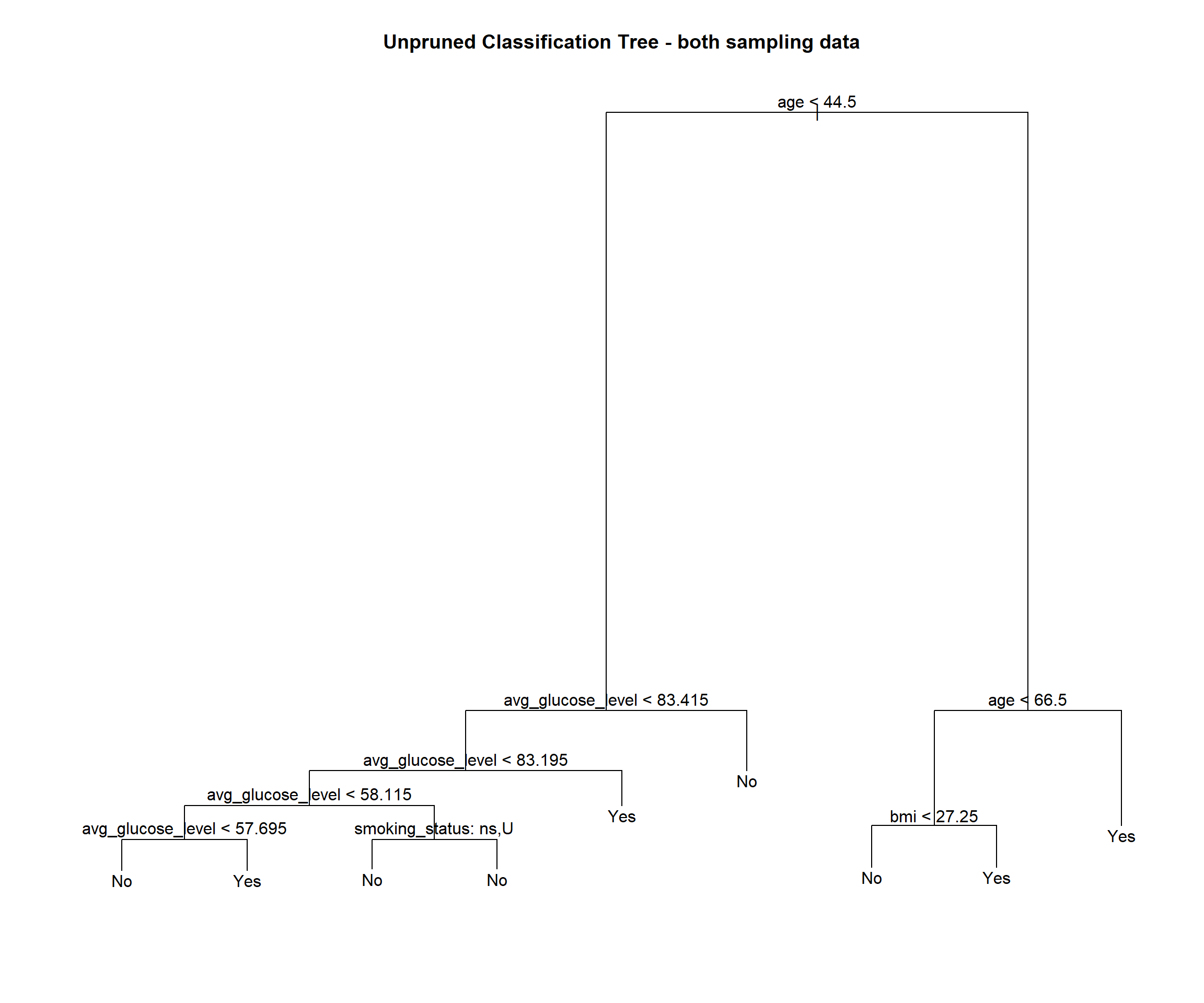
summary(stroke_tree_both)$used## [1] age avg_glucose_level smoking_status bmi
## 11 Levels: <leaf> gender age hypertension heart_disease ... smoking_statusnames(both_sampling)[which(!(names(both_sampling) %in% summary(stroke_tree_both)$used))]## [1] "gender" "hypertension" "heart_disease" "ever_married"
## [5] "work_type" "residence_type" "stroke"We see this tree has 9 terminal nodes and a misclassification rate of 0.217. The tree has only used 4 vaiables (age, smoking status, average glucose level and bmi).
confusionMatrix(predict(stroke_tree_both, both_sampling, type = "class"), both_sampling$stroke, positive = "Yes")## Confusion Matrix and Statistics
##
## Reference
## Prediction No Yes
## No 1175 80
## Yes 772 1899
##
## Accuracy : 0.783
## 95% CI : (0.7698, 0.7958)
## No Information Rate : 0.5041
## P-Value [Acc > NIR] : < 2.2e-16
##
## Kappa : 0.5647
##
## Mcnemar's Test P-Value : < 2.2e-16
##
## Sensitivity : 0.9596
## Specificity : 0.6035
## Pos Pred Value : 0.7110
## Neg Pred Value : 0.9363
## Prevalence : 0.5041
## Detection Rate : 0.4837
## Detection Prevalence : 0.6803
## Balanced Accuracy : 0.7815
##
## 'Positive' Class : Yes
## confusionMatrix(predict(stroke_tree_both, test, type = "class"), test$stroke, positive = "Yes")## Confusion Matrix and Statistics
##
## Reference
## Prediction No Yes
## No 588 4
## Yes 352 38
##
## Accuracy : 0.6375
## 95% CI : (0.6065, 0.6676)
## No Information Rate : 0.9572
## P-Value [Acc > NIR] : 1
##
## Kappa : 0.107
##
## Mcnemar's Test P-Value : <2e-16
##
## Sensitivity : 0.90476
## Specificity : 0.62553
## Pos Pred Value : 0.09744
## Neg Pred Value : 0.99324
## Prevalence : 0.04277
## Detection Rate : 0.03870
## Detection Prevalence : 0.39715
## Balanced Accuracy : 0.76515
##
## 'Positive' Class : Yes
## Here it is easy to see that the tree is a better fit than the unbalanced train model but not a better fit than over sampled (greater accuracy) and under sampled models(greater accuracy).
However the tree has been over-fit. The both sampling train set performs much better than the test set.
- This means that the under sampled tree model is the best to predict stroke with test accuracy of 66.8%, sensitivity of 80.95% and specificity of 66.17%.
4.2.2 Pruned classification tree
We will now use cross-validation to find a tree by considering trees of different sizes which have been pruned from our selected tree.
set.seed(43)
stroke_tree_under_cv = cv.tree(stroke_tree_under, FUN = prune.misclass)
stroke_tree_under_cv
## $size
## [1] 9 7 5 4 2 1
##
## $dev
## [1] 100 94 88 90 90 195
##
## $k
## [1] -Inf 0.0 0.5 5.0 6.5 83.0
##
## $method
## [1] "misclass"
##
## attr(,"class")
## [1] "prune" "tree.sequence"# index of tree with minimum error
min_idx = which.min(stroke_tree_under_cv$dev)
min_idx## [1] 3# number of terminal nodes in that tree
stroke_tree_under_cv$size[min_idx]## [1] 5# misclassification rate of each tree
stroke_tree_under_cv$dev / nrow(under_sampling)## [1] 0.2994012 0.2814371 0.2634731 0.2694611 0.2694611 0.5838323par(mfrow = c(1, 2))
# default plot
plot(stroke_tree_under_cv)
# better plot
plot(stroke_tree_under_cv$size, stroke_tree_under_cv$dev / nrow(under_sampling), type = "b",
xlab = "Tree Size", ylab = "CV Misclassification Rate")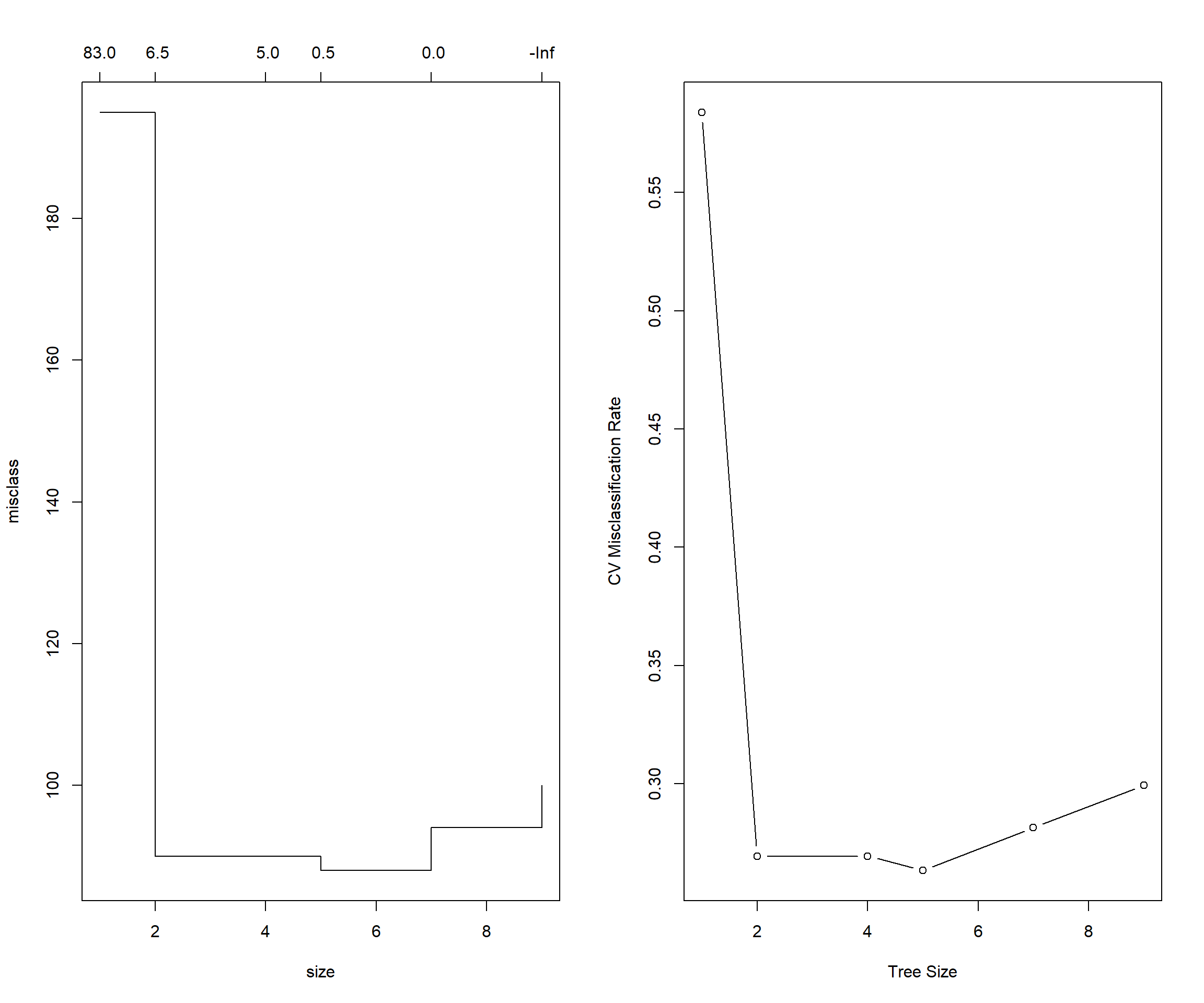
It appears that a tree of size 5 has the fewest misclassifications of the considered trees, via cross-validation.
We use prune.misclass() to obtain that tree from our selected tree, and plot this smaller tree.
stroke_tree_under_prune = prune.misclass(stroke_tree_under, best = 5)
summary(stroke_tree_under_prune)
##
## Classification tree:
## snip.tree(tree = stroke_tree_under, nodes = c(7L, 2L))
## Variables actually used in tree construction:
## [1] "age" "smoking_status" "hypertension"
## Number of terminal nodes: 5
## Residual mean deviance: 0.9302 = 306 / 329
## Misclassification error rate: 0.1976 = 66 / 334plot(stroke_tree_under_prune)
text(stroke_tree_under_prune, pretty = 0)
title(main = "Pruned Classification Tree - under sampling data")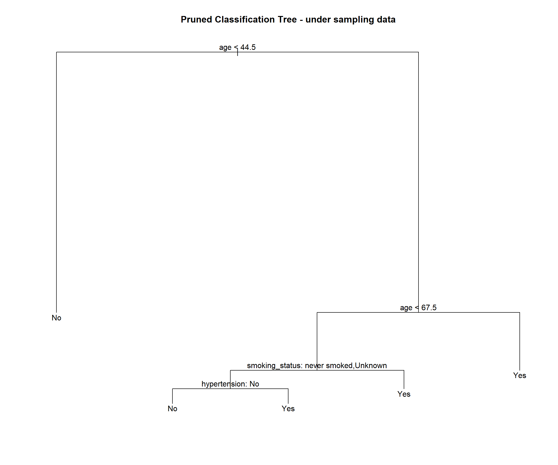
We again obtain predictions using this smaller tree, and evaluate on the test and train sets.
confusionMatrix(predict(stroke_tree_under_prune, under_sampling, type = "class"),
                under_sampling$stroke, positive = "Yes")
## Confusion Matrix and Statistics
##
## Reference
## Prediction No Yes
## No 124 23
## Yes 43 144
##
## Accuracy : 0.8024
## 95% CI : (0.7556, 0.8437)
## No Information Rate : 0.5
## P-Value [Acc > NIR] : < 2e-16
##
## Kappa : 0.6048
##
## Mcnemar's Test P-Value : 0.01935
##
## Sensitivity : 0.8623
## Specificity : 0.7425
## Pos Pred Value : 0.7701
## Neg Pred Value : 0.8435
## Prevalence : 0.5000
## Detection Rate : 0.4311
## Detection Prevalence : 0.5599
## Balanced Accuracy : 0.8024
##
## 'Positive' Class : Yes
## confusionMatrix(predict(stroke_tree_under_prune, test, type = "class"), test$stroke, positive = "Yes")## Confusion Matrix and Statistics
##
## Reference
## Prediction No Yes
## No 659 8
## Yes 281 34
##
## Accuracy : 0.7057
## 95% CI : (0.6761, 0.7341)
## No Information Rate : 0.9572
## P-Value [Acc > NIR] : 1
##
## Kappa : 0.1244
##
## Mcnemar's Test P-Value : <2e-16
##
## Sensitivity : 0.80952
## Specificity : 0.70106
## Pos Pred Value : 0.10794
## Neg Pred Value : 0.98801
## Prevalence : 0.04277
## Detection Rate : 0.03462
## Detection Prevalence : 0.32077
## Balanced Accuracy : 0.75529
##
## 'Positive' Class : Yes
## The under sampled pruned tree model has test accuracy of 70.57%, sensitivity of 80.95% and specificity of 70.11%.
There was an improvement in test set. Pruned under sampled tree model is a better fit than unpruned under sampled tree model. Test Accuracy is higher (70.57% > 66.8%), Test Sensitivity is equal (80.95%) and test Specificity is higher (70.11% > 66.17%)
It is still obvious that we have over-fit. Trees tend to do this. There are several ways to fix this, including: bagging, boosting and random forests.