Modeling COVID-19 data
1 Introduction
The COVID-19 infection, caused by the novel coronavirus SARS-CoV-2, is a contagious disease that can be transmitted through droplets, aerosols, and contact. The symptoms of COVID-19 infection appear after approximately 5.2 days (incubation period), which ranges from most common (fever, sore throat, cough, and fatigue) to variable ones (loss of smell, sputum production, headache, haemoptysis, diarrhoea, dyspnoea, and lymphopenia). In severe cases, infected cases may develop pneumonia, bronchitis, severe acute respiratory distress syndrome (ARDS), multi-organ failure, and death. The first confirmed COVID-19 case was detected in the Chinese city of Wuhan in late December 31, 2019, since then, the virus has spread worldwide. The World Health Organization (WHO) declared COVID-19 outbreak as a pandemic on March 11th, 2020. The reported cases of COVID-19 have since risen exponentially worldwide reaching more than 250 countries.
In the emergence of a new infectious disease outbreak, predicting the trend of the epidemic is of crucial importance to suggest effective control measures and estimate how contagious it is and how far it could spread. Mathematical modelling plays a key role in understanding the transmission rates and prediction evaluation of infectious diseases and their control measures. Thus, it can provide insights into the epidemiological characteristic which help decision makers to implement restriction strategies and prepare the health system capacities in the course of the pandemic.
The history of the mathematical modeling of infectious diseases greatly remounts to the study of Sir Ronald Ross in 1911 who invented a classic malaria model and also discovered the mosquito-borne transmission mechanisms of malaria.
The basic reproduction number, \(R_0\) (pronounced as R nought), is a key quantity used to estimate transmissibility of infectious diseases. If this number is equal to one or less, \(R_0\)≤1, it indicates that the number of secondary cases will decrease over time and eventually the outbreak will peter out. However, when \(R_0\)>1, the outbreak is expected as transmission to secondary cases increases that urges the implementation of control measures.
There are several different methods to estimate \(R_0\):
- Deterministic models
- Employing detailed curve fitting method assuming a structured epidemic model
- Using the intrinsic growth rate (or doubling time)
Deterministic models do not permit incorporating stochasticity explicitly (e.g. standard error for \(R_0\) is determined by measurement of errors alone), as the models argue only average number of secondary transmissions within the assumed transmission dynamics.
- Stochastic models
- Branching (Galton-Watson) process
- Counting process
2 Data Exploration
2.1 loading Relevant packages
#Import relevant packages

## tidyverse includes readr, ggplot2, dplyr, forcats, tibble, tidyr, purrr, stringr
library(tidyverse)
library(janitor)
library(lubridate)
library(plotly)
library(knitr)
2.2 loading data Set
S_I_R_V3 <- read_csv("https://raw.githubusercontent.com/reinpmomz/Data_sets/main/Data/COVID-19_12.03.2020-15.05.2021.csv")%>%
  clean_names()%>%
  select(1:18)


View(S_I_R_V3)
2.3 Cleaning the data
counties <- S_I_R_V3%>%
  select(county_where_the_case_was_diagonised)%>%
  mutate(across(c(county_where_the_case_was_diagonised), str_to_upper))%>%
  mutate(county_where_the_case_was_diagonised =
           ifelse(county_where_the_case_was_diagonised == "MALAWI", "NAIROBI",                                             county_where_the_case_was_diagonised))%>%
  drop_na()%>%
  unique()


S_I_R_V3_r <- S_I_R_V3%>%
  mutate(across(c(3:12,15,17), str_to_upper))%>%
  mutate(age_years = as.numeric(age_years))%>%
  mutate(age_years = ifelse(age_years > 110 | age_years < 1, NA, age_years))%>%
  mutate(sex = ifelse(sex == "Y", NA, sex))%>%
  mutate(date_sample_collected = dmy(date_sample_collected))%>%
  mutate(date_of_lab_confirmation = dmy(date_of_lab_confirmation))%>%
  mutate(county_where_the_case_was_diagonised =
           ifelse(county_where_the_case_was_diagonised == "MALAWI", "NAIROBI",                                             county_where_the_case_was_diagonised))%>%
  mutate(difficulty_in_breathing =
              ifelse(difficulty_in_breathing == "CHESTPAIN" , "YES",difficulty_in_breathing))%>%
  mutate(nationality = if_else(str_detect(nationality, "ZIMB"), "ZIMBABWE",
              if_else(str_detect(nationality, "KENYA")|
      str_detect(nationality, paste(c(unique(counties$county_where_the_case_was_diagonised)),
                                    collapse = "|")),"KENYA",
      if_else(str_detect(nationality, "AFGHAN"), "AFGHANISTAN",
          if_else(nationality == "AMERICAN"| nationality == "USA",
                  "UNITED STATES OF AMERICA",
        if_else(nationality == "AUSRALIAN"| nationality == "AUSTRALIA"|
                 nationality == "AUSTRARIAN", "AUSTRALIAN",
        if_else(nationality == "BRITAIN"| nationality == "BRITISH"|
               nationality == "BRITON"| nationality == "LONDON" , "UK",
        if_else(nationality == "BURKINABE", "BURKINA FASO",
  if_else(nationality == "BURUNDIAN"| nationality == "BRURUNDIAN", "BURUNDI",
      if_else(str_detect(nationality, "CAMEROON")|
                nationality == "CAMROONIAN", "CAMEROON",
    if_else(nationality == "CADIAN"| nationality == "CANDIAN"|
          nationality == "CANADAIAN"| nationality == "CANADIAN" , "CANADA",
        if_else(str_detect(nationality, "CHADIA"), "CHAD",
    if_else(nationality == "CENRAL AFRICAN"|
          nationality == "CENTRAL AFRICAN", "CENTRAL AFRICAN REPUBLIC",
          if_else(nationality == "CHINESE", "CHINA",
    if_else(nationality == "URUGUAYAN"| nationality == "URUGUYIAN", "URUGUAY",
    if_else(nationality == "UKRAIN"| nationality == "UKRAINIAN"|
               nationality == "UKRANIAN" , "UKRAINE",
     if_else(str_detect(nationality, "UGANDA"), "UGANDA",
         if_else(str_detect(nationality, "YEMEN"), "YEMEN",
             if_else(str_detect(nationality, "TUNIS"), "TUNISIA",
    if_else(nationality == "THAI", "THAILAND",
  if_else(nationality == "TRINIADADIAN"| nationality == "TRINIDADIAN", "TRINIDAD",
   if_else(nationality == "TANXANIAN"| nationality == "TANZANIAN", "TANZANIA",
  if_else(nationality == "ASWISS"| nationality == "SWISS", "SWITZERLAND",
  if_else(nationality == "SWDISH"| nationality == "SWEDISH", "SWEDEN",
   if_else(nationality == "SUDANESE"| nationality == "SUDANESSE", "SUDAN",
  if_else(nationality == "SOUTH SUDANASE"|
            nationality == "SOUTH SUDANESE", "SOUTH SUDAN",
  if_else(nationality == "SRI LANAKAN"| nationality == "SIRI LANKAN"|
            nationality == "SRI LANKAN", "SRI LANKA",
    if_else(nationality == "SOTH AFRICAN"|
            nationality == "SOUTH AFRICAN", "SOUTH AFRICA",
    if_else(str_detect(nationality, "SOMALI"), "SOMALIA",
    if_else(nationality == "SIERRA LEONEAN"| nationality == "SIERRA LEONIAN"|
               nationality == "SIERRA LEONNE"|
              nationality == "SUIERRA LEONNE", "SIERRA LEONE",
    if_else(str_detect(nationality, "RWAND")| nationality == "RWADESE",
            "RWANDA",
    if_else(str_detect(nationality, "ROMANIA"), "ROMANIA",
    if_else(str_detect(nationality, "PORTUG"), "PORTUGAL",
      if_else(nationality == "PRUVIAN"|nationality == "PERUVIAN", "PERU",
    if_else(nationality == "PHILLIPINO"| nationality == "FILIPINO"|
            nationality == "FILIPO"| nationality == "FILLIPINO",
            "PHILIPPINES",
    if_else(nationality == "PAKISTANI"|nationality == "PAKSITANI"|
             nationality == "PAKSTANI" , "PAKISTAN",
                                nationality
        ))))))))))))))))))))))))))))))))))))


S_I_R_V3_final <- S_I_R_V3_r%>%
  mutate(nationality = if_else(str_detect(nationality, "NIGERI"), "NIGERIA",
      if_else(str_detect(nationality, "NEW ZE"), "NEW ZEALAND",
              if_else(nationality == "NI-VANUATU", "VANUATU",
      if_else(nationality == "MOZABICAN", "MOZAMBICAN",
      if_else(nationality == "MOTSWANA", "BOTSWANA",
      if_else(nationality == "MOSOTHO", "LESOTHO",
    if_else(nationality == "MEXICAN"| nationality == "MERXICAN", "MEXICO",
    if_else(str_detect(nationality, "MALAWI"), "MALAWI",
    if_else(str_detect(nationality, "KUWAIT"), "KUWAIT",
    if_else(nationality == "MALASYIAN"| nationality == "MALAYSIAN"|
      nationality == "MALYSIAN"| nationality == "MARASIA","MALAYSIA",
     if_else(nationality == "LITHUNIAN", "LITHUANIAN",
    if_else(nationality == "LABANESE"| nationality == "LEBENESE", "LEBANESE",
    if_else(nationality == "KITTITIAN", "SAINT KITTS AND NEVIS",
    if_else(nationality == "KOREAN", "SOUTH KOREAN",
    if_else(str_detect(nationality, "KAZAKH"), "KAZAKHSTAN",
    if_else(str_detect(nationality, "JAPAN"), "JAPAN",
     if_else(str_detect(nationality, "ITALY"), "ITALIAN",
    if_else(nationality == "ISRAEL"| nationality == "ISREAL", "ISRAELI",
    if_else(nationality == "IRARIAN", "IRANIAN",
    if_else(nationality == "INDIIAN"| nationality == "INDIA"|
              nationality == "ASIAN", "INDIAN",
    if_else(str_detect(nationality, "BANGLADESH")|nationality == "BENGALI" ,
            "BANGLADESH",
        if_else(nationality == "BELGIAN", "BELGIUM",
        if_else(str_detect(nationality, "BRAZIL"), "BRAZIL",
        if_else(str_detect(nationality, "KIRIBATI"), "KIRIBATI",
  if_else(nationality == "GHANANIAN"| nationality == "GHANIAN", "GHANAIAN",
  if_else(nationality == "GERAMAN"| nationality == "GERMANY", "GERMAN",
  if_else(str_detect(nationality, "ETHIO")| nationality == "ETHIPIAN", "ETHIOPIA",
  if_else(str_detect(nationality, "ERITREA")| nationality == "ERITERIAN" |
          nationality == "ERTREAN" , "ERITREAN",
  if_else(nationality == "EMARATI"| nationality == "EMIRATI", "U.A.E",
  if_else(str_detect(nationality, "DJIBOUTI")| nationality == "EMARATI",
          "DJBOUTIAN",
      if_else(nationality == "CHZEN", "CZECH",
       if_else(str_detect(nationality, "COMOR"), "COMOROS",
                                nationality )))))))))))))))))))))))))))))))))%>%
  mutate(lab_results = ifelse(str_detect(lab_results, "POSIT")|
                        lab_results == "POSTIVE", "POSITIVE",
                              NA))%>%
  replace_na(list(lab_results = "POSITIVE"))%>%
  mutate(outcome_death_discharge_still_in_hospital =
        ifelse(outcome_death_discharge_still_in_hospital == "44303", NA,
                  outcome_death_discharge_still_in_hospital))%>%
  mutate(recovered =
      if_else(outcome_death_discharge_still_in_hospital == "DEAD"|
      outcome_death_discharge_still_in_hospital == "STILL IN HOSPITAL","NO",
      "YES"))%>%
  replace_na(list(recovered = "YES"))%>%
  mutate(deaths =
      if_else(outcome_death_discharge_still_in_hospital == "DEAD","YES",
      "NO"))%>%
  replace_na(list(deaths = "NO"))
3 Epidemic curves
3.1 Countrywide
date_cases_plot <- tibble(date = c(seq(min(S_I_R_V3_final$date_of_lab_confirmation), max(S_I_R_V3_final$date_of_lab_confirmation), by=1)))%>%
  left_join(S_I_R_V3_final%>%
  select(date_of_lab_confirmation, lab_results,
         deaths)%>%
    mutate(deaths = ifelse(deaths == "YES" , 1, 0))%>%
  group_by(date_of_lab_confirmation)%>%
  summarise(cases = length(lab_results),
            deaths = sum(deaths), .groups = "drop"),
  by = c("date" = "date_of_lab_confirmation"))%>%
  replace_na(list(cases = 0))%>%
  replace_na(list(deaths = 0))%>%
  mutate(total_cases = cumsum(cases))%>%
  mutate(total_deaths= cumsum(deaths))


week_date_cases_plot <- date_cases_plot%>%
                       mutate(week_year = ceiling_date(date, unit = "week"))%>%
  group_by(week_year)%>%
  summarise(cases = sum(cases),
            deaths = sum(deaths), .groups = "drop")%>%
  mutate(total_cases = cumsum(cases))%>%
  mutate(total_deaths= cumsum(deaths))


month_date_cases_plot <- date_cases_plot%>%
                       mutate(month_year = floor_date(date, unit = "month"))%>%
  group_by(month_year)%>%
  summarise(cases = sum(cases),
            deaths = sum(deaths), .groups = "drop")%>%
  mutate(total_cases = cumsum(cases))%>%
  mutate(total_deaths= cumsum(deaths))
From 2020-03-12 to 2021-05-15, there was a total of 165465 cases and 3003 deaths.
3.1.1 Daily trend
library(reshape2)

plot_ly(data=melt(date_cases_plot, id=c("date", "total_cases", "total_deaths")),
                x = ~date, y = ~value ,
                type = 'scatter', mode = 'lines', line = list( width=1.5),
        color = ~variable, colors = c("orange", "red"))%>%
  layout( title = list( text = "<b> Daily Trend of COVID-19 <b>",
                      font = list(size = 18),
              y = 0.99, x = 0.5, xanchor = 'center', yanchor =  'top' ),
          hovermode = "x unified",
          yaxis = list(title = 'Total No.',
                                     gridcolor = 'lightgrey',
                                     titlefont = list(size = 16, color = '#000000'),
                                     tickfont = list(size = 14, color = 'black'),
                                     tickformat = "digits",
                                     tickangle=0,
                                     nticks=15),
                        xaxis = list(title = 'Days',
                                     type = 'date',
                                     tickformat = "%d %b %Y",
                                     gridcolor = 'lightgrey',
                                     titlefont = list(size = 16, color = '#000000'),
                                     tickfont = list(size = 14, color = 'black'),
                                     tickangle=-45),
          range=c(min(date_cases_plot$date)-days(5),
                                             max(date_cases_plot$date)+days(2)))
The day with highest number of cases was 2021-03-25 with 2022 cases.
The day with highest number of deaths was 2021-03-25, 2021-03-29 with 35 deaths.
3.1.2 Weekly trend
plot_ly(data=melt(week_date_cases_plot, id=c("week_year", "total_cases", "total_deaths")),
                x = ~week_year, y = ~value ,
                type = 'scatter', mode = 'lines', line = list( width=1.5),
        color = ~variable, colors = c("orange", "red"))%>%
  layout( title = list( text = "<b> Weekly Trend of COVID-19 <b>",
                      font = list(size = 18),
              y = 0.99, x = 0.5, xanchor = 'center', yanchor =  'top' ),
          hovermode = "x unified",
          yaxis = list(title = 'Total No.',
                                     gridcolor = 'lightgrey',
                                     titlefont = list(size = 16, color = '#000000'),
                                     tickfont = list(size = 14, color = 'black'),
                                     tickformat = "digits",
                                     tickangle=0,
                                     nticks=15),
                        xaxis = list(title = 'Weeks',
                                     type = 'date',
                                     tickformat = "%d %b %Y",
                                     gridcolor = 'lightgrey',
                                     titlefont = list(size = 16, color = '#000000'),
                                     tickfont = list(size = 14, color = 'black'),
                                     tickangle=-45),
          range=c(min(date_cases_plot$date)-days(5),
                                             max(date_cases_plot$date)+days(2)))
3.1.3 Monthly trend
plot_ly(data=melt(month_date_cases_plot, id=c("month_year", "total_cases", "total_deaths")),
                x = ~month_year, y = ~value ,
                type = 'scatter', mode = 'lines', line = list( width=1.5),
        color = ~variable, colors = c("orange", "red"))%>%
  layout( title = list( text = "<b> Monthly Trend of COVID-19 <b>",
                      font = list(size = 18),
              y = 0.99, x = 0.5, xanchor = 'center', yanchor =  'top' ),
          hovermode = "x unified",
          yaxis = list(title = 'Total No.',
                                     gridcolor = 'lightgrey',
                                     titlefont = list(size = 16, color = '#000000'),
                                     tickfont = list(size = 14, color = 'black'),
                                     tickformat = "digits",
                                     tickangle=0,
                                     nticks=15),
                        xaxis = list(title = 'Months',
                                     type = 'date',
                                     tickformat = "%b %Y",
                                     gridcolor = 'lightgrey',
                                     titlefont = list(size = 16, color = '#000000'),
                                     tickfont = list(size = 14, color = 'black'),
                                     tickangle=-45),
          range=c(min(date_cases_plot$date)-days(5),
                                             max(date_cases_plot$date)+days(2)))
The month with highest number of cases was 2021-03-01 with 29035 cases.
The month with highest number of deaths was 2021-03-01 with 526 deaths.
3.1.4 Cummulative trend
plot_ly(data=melt(date_cases_plot, id=c("date", "cases", "deaths")),
                x = ~date, y = ~value ,
                type = 'scatter', mode = 'lines', line = list( width=1.5),
        color = ~variable, colors = c("orange", "red"))%>%
  layout( title = list( text = "<b> Cummulative Trend of COVID-19 <b>",
                      font = list(size = 18),
              y = 0.99, x = 0.5, xanchor = 'center', yanchor =  'top' ),
          hovermode = "x unified",
          yaxis = list(title = 'Total No.',
                                     gridcolor = 'lightgrey',
                                     titlefont = list(size = 16, color = '#000000'),
                                     tickfont = list(size = 14, color = 'black'),
                                     tickformat = "digits",
                                     tickangle=0,
                                     nticks=15),
                        xaxis = list(title = 'Days',
                                     type = 'date',
                                     tickformat = "%d %b %Y",
                                     gridcolor = 'lightgrey',
                                     titlefont = list(size = 16, color = '#000000'),
                                     tickfont = list(size = 14, color = 'black'),
                                     tickangle=-45),
          range=c(min(date_cases_plot$date)-days(5),
                                             max(date_cases_plot$date)+days(2)))
plot_ly(date_cases_plot, hoverinfo = "text+y+name"
,text = ~paste(format(date, format = "%d %b, %Y"))
)%>%
add_trace(x = ~date, y = ~total_cases, type = 'scatter', mode = 'lines',
name = 'Total Cases',line = list(color= 'orange', width=1.5)
)%>%
add_trace(x = ~date, y = ~total_deaths, type = 'scatter', mode = 'lines',
name = 'Total Deaths', yaxis = 'y2',line = list(color= 'red', width=1.5)
)%>%
layout(title = list (text = "<b> Cummulative Trend of COVID-19 <b>",
font = list(size = 18),
y = 0.99, x = 0.5, xanchor = 'center', yanchor = 'top'),
hovermode = "x unified",
legend = list(orientation = 'v', x= 1.07, y=1),
xaxis = list(title = "Days", range=c(min(date_cases_plot$date)-days(5),
max(date_cases_plot$date)+days(5)),
type = 'date',
tickformat = "%d %b %Y",
gridcolor = 'lightgrey',
titlefont = list(size = 16, color = '#000000'),
tickfont = list(size = 14, color = 'black'),
tickangle=-45),
yaxis = list(side = 'left', title = 'Total Cases', tickformat = "digits",
showgrid = FALSE, zeroline = FALSE,
titlefont = list(size = 16, color = '#000000'),
tickfont = list(size = 14, color = 'black'),
tickangle=0,
nticks=10),
yaxis2 = list(side = 'right', overlaying = "y", title = 'Total Deaths',
tickformat = "digits",
showgrid = FALSE, zeroline = FALSE,
titlefont = list(size = 16, color = 'blue'),
tickfont = list(size = 14, color = 'darkblue'),
tickangle=0,
nticks=10))3.2 County
date_cases_plot_county <- do.call("rbind",
                                  replicate(47, date_cases_plot%>%dplyr::select(date),
                                            simplify = FALSE))%>%
  mutate(county = rep(c(unique(counties$county_where_the_case_was_diagonised)),
                         each = 430, times = 1))%>%
  left_join(S_I_R_V3_final%>%
  select(county_where_the_case_was_diagonised, date_of_lab_confirmation, lab_results,
         deaths)%>%
    mutate(deaths = ifelse(deaths == "YES" , 1, 0))%>%
  group_by(county_where_the_case_was_diagonised, date_of_lab_confirmation)%>%
  summarise(cases = length(lab_results),
            deaths = sum(deaths), .groups = "drop"),
  by = c("date" = "date_of_lab_confirmation",
         "county" = "county_where_the_case_was_diagonised"))%>%
  replace_na(list(cases = 0))%>%
  replace_na(list(deaths = 0))%>%
  group_by(county)%>%
  mutate(total_cases = cumsum(cases))%>%
  mutate(total_deaths= cumsum(deaths))%>%
  ungroup()


week_date_cases_plot_county <- date_cases_plot_county%>%
                       mutate(week_year = lubridate::ceiling_date(date, unit = "week"))%>%
  group_by(county, week_year)%>%
  summarise(cases = sum(cases),
            deaths = sum(deaths), .groups = "drop")%>%
  group_by(county)%>%
  mutate(total_cases = cumsum(cases))%>%
  mutate(total_deaths= cumsum(deaths))%>%
  ungroup()


month_date_cases_plot_county <- date_cases_plot_county%>%
                       mutate(month_year = floor_date(date, unit = "month"))%>%
  group_by(county, month_year)%>%
  summarise(cases = sum(cases),
            deaths = sum(deaths), .groups = "drop")%>%
  group_by(county)%>%
  mutate(total_cases = cumsum(cases))%>%
  mutate(total_deaths= cumsum(deaths))%>%
  ungroup()
3.2.1 Daily trend
plot_ly(date_cases_plot_county,
                x = ~date, y = ~cases ,
                type = 'scatter', mode = 'lines', color = ~county)%>%
  layout( title = list( text = "<b> Daily County Trend of COVID-19 cases <b>",
                      font = list(size = 18),
              y = 0.99, x = 0.5, xanchor = 'center', yanchor =  'top' ),
          yaxis = list(title = 'Total No.',
                                     gridcolor = 'lightgrey',
                                     titlefont = list(size = 16, color = '#000000'),
                                     tickfont = list(size = 14, color = 'black'),
                                     tickformat = "digits",
                                     tickangle=0,
                                     nticks=10),
                        xaxis = list(title = 'Days',
                                     type = 'date',
                                     tickformat = "%d %b %Y",
                                     gridcolor = 'lightgrey',
                                     titlefont = list(size = 16, color = '#000000'),
                                     tickfont = list(size = 14, color = 'black'),
                                     tickangle=-45))
plot_ly(date_cases_plot_county,
x = ~date, y = ~deaths,
type = 'scatter', mode = 'lines', color = ~county)%>%
layout( title = list( text = "<b> Daily County Trend of COVID-19 deaths <b>",
font = list(size = 18),
y = 0.99, x = 0.5, xanchor = 'center', yanchor = 'top' ),
yaxis = list(title = 'Total No.',
gridcolor = 'lightgrey',
titlefont = list(size = 16, color = '#000000'),
tickfont = list(size = 14, color = 'black'),
tickformat = "digits",
tickangle=0,
nticks=10),
xaxis = list(title = 'Days',
type = 'date',
tickformat = "%d %b %Y",
gridcolor = 'lightgrey',
titlefont = list(size = 16, color = '#000000'),
tickfont = list(size = 14, color = 'black'),
tickangle=-45))3.2.2 Weekly trend
plot_ly(week_date_cases_plot_county,
                x = ~week_year, y = ~cases ,
                type = 'scatter', mode = 'lines', color = ~county)%>%
  layout( title = list( text = "<b> Weekly County Trend of COVID-19 cases <b>",
                      font = list(size = 18),
              y = 0.99, x = 0.5, xanchor = 'center', yanchor =  'top' ),
          yaxis = list(title = 'Total No.',
                                     gridcolor = 'lightgrey',
                                     titlefont = list(size = 16, color = '#000000'),
                                     tickfont = list(size = 14, color = 'black'),
                                     tickformat = "digits",
                                     tickangle=0,
                                     nticks=10),
                        xaxis = list(title = 'Weeks',
                                     type = 'date',
                                     tickformat = "%d %b %Y",
                                     gridcolor = 'lightgrey',
                                     titlefont = list(size = 16, color = '#000000'),
                                     tickfont = list(size = 14, color = 'black'),
                                     tickangle=-45))
plot_ly(week_date_cases_plot_county,
x = ~week_year, y = ~deaths,
type = 'scatter', mode = 'lines', color = ~county)%>%
layout( title = list( text = "<b> Weekly County Trend of COVID-19 deaths <b>",
font = list(size = 18),
y = 0.99, x = 0.5, xanchor = 'center', yanchor = 'top' ),
yaxis = list(title = 'Total No.',
gridcolor = 'lightgrey',
titlefont = list(size = 16, color = '#000000'),
tickfont = list(size = 14, color = 'black'),
tickformat = "digits",
tickangle=0,
nticks=10),
xaxis = list(title = 'Weeks',
type = 'date',
tickformat = "%d %b %Y",
gridcolor = 'lightgrey',
titlefont = list(size = 16, color = '#000000'),
tickfont = list(size = 14, color = 'black'),
tickangle=-45))3.2.3 Monthly trend
plot_ly(month_date_cases_plot_county,
                x = ~month_year, y = ~cases ,
                type = 'scatter', mode = 'lines', color = ~county)%>%
  layout( title = list( text = "<b> Monthly County Trend of COVID-19 cases <b>",
                      font = list(size = 18),
              y = 0.99, x = 0.5, xanchor = 'center', yanchor =  'top' ),
          yaxis = list(title = 'Total No.',
                                     gridcolor = 'lightgrey',
                                     titlefont = list(size = 16, color = '#000000'),
                                     tickfont = list(size = 14, color = 'black'),
                                     tickformat = "digits",
                                     tickangle=0,
                                     nticks=10),
                        xaxis = list(title = 'Months',
                                     type = 'date',
                                     tickformat = "%b %Y",
                                     gridcolor = 'lightgrey',
                                     titlefont = list(size = 16, color = '#000000'),
                                     tickfont = list(size = 14, color = 'black'),
                                     tickangle=-45))
plot_ly(month_date_cases_plot_county,
x = ~month_year, y = ~deaths,
type = 'scatter', mode = 'lines', color = ~county)%>%
layout( title = list( text = "<b> Monthly County Trend of COVID-19 deaths <b>",
font = list(size = 18),
y = 0.99, x = 0.5, xanchor = 'center', yanchor = 'top' ),
yaxis = list(title = 'Total No.',
gridcolor = 'lightgrey',
titlefont = list(size = 16, color = '#000000'),
tickfont = list(size = 14, color = 'black'),
tickformat = "digits",
tickangle=0,
nticks=10),
xaxis = list(title = 'Months',
type = 'date',
tickformat = "%b %Y",
gridcolor = 'lightgrey',
titlefont = list(size = 16, color = '#000000'),
tickfont = list(size = 14, color = 'black'),
tickangle=-45))3.2.4 Cummulative trend
plot_ly(date_cases_plot_county,
                x = ~date, y = ~total_cases ,
                type = 'scatter', mode = 'lines', color = ~county)%>%
  layout( title = list( text = "<b> Cummulative County Trend of COVID-19 cases <b>",
                      font = list(size = 18),
              y = 0.99, x = 0.5, xanchor = 'center', yanchor =  'top' ),
          yaxis = list(title = 'Total No.',
                                     gridcolor = 'lightgrey',
                                     titlefont = list(size = 16, color = '#000000'),
                                     tickfont = list(size = 14, color = 'black'),
                                     tickformat = "digits",
                                     tickangle=0,
                                     nticks=10),
                        xaxis = list(title = 'Days',
                                     type = 'date',
                                     tickformat = "%d %b %Y",
                                     gridcolor = 'lightgrey',
                                     titlefont = list(size = 16, color = '#000000'),
                                     tickfont = list(size = 14, color = 'black'),
                                     tickangle=-45))
plot_ly(date_cases_plot_county,
x = ~date, y = ~total_deaths,
type = 'scatter', mode = 'lines', color = ~county)%>%
layout( title = list( text = "<b> Cummulative County Trend of COVID-19 deaths <b>",
font = list(size = 18),
y = 0.99, x = 0.5, xanchor = 'center', yanchor = 'top' ),
yaxis = list(title = 'Total No.',
gridcolor = 'lightgrey',
titlefont = list(size = 16, color = '#000000'),
tickfont = list(size = 14, color = 'black'),
tickformat = "digits",
tickangle=0,
nticks=10),
xaxis = list(title = 'Days',
type = 'date',
tickformat = "%d %b %Y",
gridcolor = 'lightgrey',
titlefont = list(size = 16, color = '#000000'),
tickfont = list(size = 14, color = 'black'),
tickangle=-45))4 Infectious Disease Modelling
The goal of infectious disease modelling is to capture transmission dynamics. They are mathematical descriptions of the spread of infection driven by the host which then passes the infection to other individuals.
Using the model, it’s possible to:
- Study the effect of interventions on the burden of a disease.
- To project the outcome of different interventions
In infectious disease modelling, we use Compartmental models. They are a modelling approach where the population is divided into different ‘compartments’, representing their disease status and possibly other characteristics. Here, mathematical equations are used to model transitions between different compartments.
Compartmental models are divide into
- A simple two compartment model
- Sir Models
4.1 Classical (Basic/Simple) Sir Model
The classical SIR model introduced by Kermack and Mckendrick (1927) is a compartmental model where the individuals belong to one of the three compartments:
- Susceptible (S)
- Infected (I)
- Recovered (R)
It’s a population-based model in the sense that each compartment models the behavior of an average individual in that compartment.

The assumptions of the model are as follows:
- Homogeneous population : Individuals in the same compartment is subject to the same hazards
- Well-mixed population : All susceptible have the same risk of getting infected
- Immunity forever : Individuals who recovered from the disease are immune forever
- At the start of the epidemic, there is only one infected individual and no one has recovered yet.
- Closed population : Total population size which is constant (i.e. a population without immigration and emmigration)
- Background demographic processes are not included : Time-scale of the epidemic is much faster than characteristic times for demographic processes (natural birth rate and death rate).
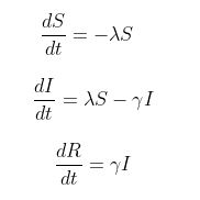
These assumptions give us the following system of nonlinear ordinary differential equations (ODEs):
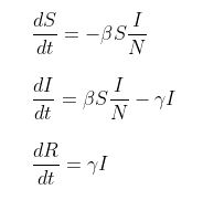
Where S, I and R represents the number of susceptible, infected and recovered individuals at time t in each compartment respectively; γ is the recovery rate; β is the infection (transmission) rate i.e the average number of secondary infections per unit time; N is the total population size and N=S+I+R.
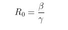
Basic Reproduction Number (\(R_0\)) - It is the average number of secondary infections caused by a single primary (infected) case, in a fully susceptible population. For an SIR model, it can be calculated as :
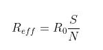
Effective Reproduction Number (\(R_{eff}\)) - It is the average number of secondary cases arising from an infected case at a given point in the epidemic. If the population of susceptible varies with time, it’s preferable to use the effective reproduction number.
Force of infection (λ) - It is the risk of infection of an individual, per unit time. It can be expressed as :
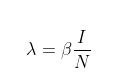
Substituting this expression for λ in the differential equations above, we obtain:
We can consider two cases for SIR models : i) SIR model with constant λ ii) SIR model with varying λ
There are also several extensions of classical sir model by factors called modifiers of susceptibility in a population. They are:
- Population turnover
- Vaccination effects
- Waning immunity
To estimate \(R_o\), we use an estimation procedure (least-square fitting) and compute the residual sum of squares for the reported cases (observed) and model cases(fitted).
4.1.1 One-Parameter Estimation (Recovery rate estimated to be 14 days)
One-dimensional optimization by Nelder-Mead is unreliable: use “Brent” or optimize() directly. Method = “Brent” is only available for one-dimensional optimization.
library(deSolve)Pop_kenya <- read_csv("https://raw.githubusercontent.com/reinpmomz/Data_sets/main/Data/V1_T2.2.csv")%>%
clean_names()%>%
filter(county == "Total")date_cases_sir <- tibble(date = c(seq(min(S_I_R_V3_final$date_of_lab_confirmation), max(S_I_R_V3_final$date_of_lab_confirmation), by=1)))%>%
left_join(S_I_R_V3_final%>%
select(date_of_lab_confirmation, lab_results,
deaths, recovered)%>%
mutate(deaths = ifelse(deaths == "YES" , 1, 0))%>%
mutate(recovered = ifelse(recovered == "YES" , 1, 0))%>%
group_by(date_of_lab_confirmation)%>%
summarise(cases = length(lab_results),
deaths = sum(deaths),
recovered = sum(recovered),.groups = "drop"),
by = c("date" = "date_of_lab_confirmation"))%>%
replace_na(list(cases = 0))%>%
replace_na(list(deaths = 0))%>%
replace_na(list(recovered = 0))%>%
mutate(status = c(
rep("Beginning",length(seq(as.Date("2020/03/12"), as.Date("2020/03/26"), by=1))),
rep("Total Lockdown",length(seq(as.Date("2020/03/27"), as.Date("2020/08/31"), by=1))),
rep("Partially opening",length(seq(as.Date("2020/09/01"), as.Date("2020/12/31"), by=1))),
rep("Reopening",length(seq(as.Date("2021/01/01"), as.Date("2021/05/15"), by=1)))))%>%
mutate(month_year_date = floor_date(date, unit = "month"))SIR_1 <- function(time, state, parameters) {
par <- as.list(c(state, parameters))
with(par, {
N=S+I+R
gamma=1/14
dS <- - (beta/N) * I * S
dI <- beta/N * I * S - gamma * I
dR <- gamma * I
list(c(dS, dI, dR))
})
}4.1.1.1 Countrywide
4.1.1.1.1 March 2020 - May 2021
RSS_Mar20_May21_beta <- function(parameters) {
  names(parameters) <- c("beta")
  initial_state_values=c(S=as.numeric(Pop_kenya$total[Pop_kenya$county == "Total"])-1,I=1,R=0)
  time=seq(from=1,
         to=length(seq(min(date_cases_sir$date), max(date_cases_sir$date), by=1))
         ,by=1)
  out <- ode(y = initial_state_values, times = time, func = SIR_1, parms = parameters)
  fit <- out[ , 3]
  sum((date_cases_sir$cases - fit)^2)
}


opt_Mar20_May21_beta <- optim(c(0.5), RSS_Mar20_May21_beta, method = "Brent", lower = 0, upper = 1)

opt_Mar20_May21_par_beta <- setNames(opt_Mar20_May21_beta$par, c("beta"))


opt_Mar20_May21_par_Ro <- setNames(opt_Mar20_May21_par_beta[1]/(1/14), "Ro" )
4.1.1.1.2 Beginning
RSS_Beginning_beta <- function(parameters) {
  names(parameters) <- c("beta")
  initial_state_values=c(S=as.numeric(Pop_kenya$total[Pop_kenya$county == "Total"])-1,I=1,R=0)
  time=seq(from=1,
         to=length(seq(min(date_cases_sir$date[which(date_cases_sir$status == "Beginning")]),
                  max(date_cases_sir$date[which(date_cases_sir$status == "Beginning")]), by=1))
         ,by=1)
  out <- ode(y = initial_state_values, times = time, func = SIR_1, parms = parameters)
  fit <- out[ , 3]
  sum((date_cases_sir$cases[date_cases_sir$status == "Beginning"] - fit)^2)
}


opt_Beginning_beta <- optim(c(0.5), RSS_Beginning_beta, method = "Brent", lower = 0, upper = 1)

opt_Beginning_par_beta <- setNames(opt_Beginning_beta$par, c("beta"))


opt_Beginning_par_Ro <- setNames(opt_Beginning_par_beta[1]/(1/14), "Ro" )
4.1.1.1.3 Total Lockdown
RSS_TotalLockdown_beta <- function(parameters) {
  names(parameters) <- c("beta")
  initial_state_values=c(S=as.numeric(Pop_kenya$total[Pop_kenya$county == "Total"]- sum(date_cases_sir$cases[which(date_cases_sir$status == "Beginning")]))-1,I=1,R=0)
  time=seq(from=1,
         to=length(seq(min(date_cases_sir$date[which(date_cases_sir$status == "Total Lockdown")]),
                  max(date_cases_sir$date[which(date_cases_sir$status == "Total Lockdown")]), by=1))
         ,by=1)
  out <- ode(y = initial_state_values, times = time, func = SIR_1, parms = parameters)
  fit <- out[ , 3]
  sum((date_cases_sir$cases[date_cases_sir$status == "Total Lockdown"] - fit)^2)
}


opt_TotalLockdown_beta <- optim(c(0.5), RSS_TotalLockdown_beta, method = "Brent", lower = 0, upper = 1)

opt_TotalLockdown_par_beta <- setNames(opt_TotalLockdown_beta$par, c("beta"))


opt_TotalLockdown_par_Ro <- setNames(opt_TotalLockdown_par_beta[1]/(1/14), "Ro" )
4.1.1.1.4 Partially opening
RSS_Partiallyopening_beta <- function(parameters) {
  names(parameters) <- c("beta")
    initial_state_values=c(
      S=as.numeric(Pop_kenya$total[Pop_kenya$county == "Total"]- sum(date_cases_sir$cases[which(date_cases_sir$status == "Beginning"|
            date_cases_sir$status == "Total Lockdown")]))-1,
      I=1,
      R=0)
  time=seq(from=1,
         to=length(seq(min(date_cases_sir$date[which(date_cases_sir$status == "Partially opening")]), max(date_cases_sir$date[which(date_cases_sir$status == "Partially opening")]), by=1))
         ,by=1)
  out <- ode(y = initial_state_values, times = time, func = SIR_1, parms = parameters)
  fit <- out[ , 3]
  sum((date_cases_sir$cases[date_cases_sir$status == "Partially opening"] - fit)^2)
}


opt_Partiallyopening_beta <- optim(c(0.5), RSS_Partiallyopening_beta, method = "Brent", lower = 0, upper = 1)

opt_Partiallyopening_par_beta <- setNames(opt_Partiallyopening_beta$par, c("beta"))


opt_Partiallyopening_par_Ro <- setNames(opt_Partiallyopening_par_beta[1]/(1/14), "Ro" )
4.1.1.1.5 Reopening
RSS_Reopening_beta <- function(parameters) {
  names(parameters) <- c("beta")
    initial_state_values=c(
      S=as.numeric(Pop_kenya$total[Pop_kenya$county == "Total"]- sum(date_cases_sir$cases[which(date_cases_sir$status == "Beginning"|
            date_cases_sir$status == "Total Lockdown"|
            date_cases_sir$status == "Partially opening")]))-1,
      I=1,
      R=0)
  time=seq(from=1,
         to=length(seq(min(date_cases_sir$date[which(date_cases_sir$status == "Reopening")]), max(date_cases_sir$date[which(date_cases_sir$status == "Reopening")]), by=1))
         ,by=1)
  out <- ode(y = initial_state_values, times = time, func = SIR_1, parms = parameters)
  fit <- out[ , 3]
  sum((date_cases_sir$cases[date_cases_sir$status == "Reopening"] - fit)^2)
}


opt_Reopening_beta <- optim(c(0.5), RSS_Reopening_beta, method = "Brent", lower = 0, upper = 1)

opt_Reopening_par_beta <- setNames(opt_Reopening_beta$par, c("beta"))


opt_Reopening_par_Ro <- setNames(opt_Reopening_par_beta[1]/(1/14), "Ro" )
4.1.1.1.6 Table Report
        kable (
          tibble(
  status= c("All", "Beginning" ,"Total Lockdown", "Partially opening", "Reopening"),
  period = c(paste0(min(date_cases_sir$date)," to ", max(date_cases_sir$date)),
             paste0(min(date_cases_sir$date[which(date_cases_sir$status == "Beginning")])," to ",               max(date_cases_sir$date[which(date_cases_sir$status == "Beginning")])),
             paste0(min(date_cases_sir$date[which(date_cases_sir$status == "Total Lockdown")])," to ",               max(date_cases_sir$date[which(date_cases_sir$status == "Total Lockdown")])),
            paste0(min(date_cases_sir$date[which(date_cases_sir$status == "Partially opening")])," to ",             max(date_cases_sir$date[which(date_cases_sir$status == "Partially opening")])),
             paste0(min(date_cases_sir$date[which(date_cases_sir$status == "Reopening")])," to ",                   max(date_cases_sir$date[which(date_cases_sir$status == "Reopening")]))),
  "n (days)" = c(length(seq(min(date_cases_sir$date), max(date_cases_sir$date), by=1)),
              length(seq(min(date_cases_sir$date[which(date_cases_sir$status == "Beginning")]),
              max(date_cases_sir$date[which(date_cases_sir$status == "Beginning")]), by=1)),
              length(seq(min(date_cases_sir$date[which(date_cases_sir$status == "Total Lockdown")]),
              max(date_cases_sir$date[which(date_cases_sir$status == "Total Lockdown")]), by=1)),
              length(seq(min(date_cases_sir$date[which(date_cases_sir$status == "Partially opening")]),
              max(date_cases_sir$date[which(date_cases_sir$status == "Partially opening")]), by=1)),
              length(seq(min(date_cases_sir$date[which(date_cases_sir$status == "Reopening")]),
              max(date_cases_sir$date[which(date_cases_sir$status == "Reopening")]), by=1))),
  "Gamma (Recovery rate)" = c(rep(round(1/14, 4),5)),
  "Beta (Infection rate)" = round(c(opt_Mar20_May21_par_beta, opt_Beginning_par_beta,
                                    opt_TotalLockdown_par_beta,
                              opt_Partiallyopening_par_beta, opt_Reopening_par_beta),4),
  "Ro" = round(c(opt_Mar20_May21_par_Ro, opt_Beginning_par_Ro, opt_TotalLockdown_par_Ro,
           opt_Partiallyopening_par_Ro, opt_Reopening_par_Ro ),4),
  )
)| status | period | n (days) | Gamma (Recovery rate) | Beta (Infection rate) | Ro |
|---|---|---|---|---|---|
| All | 2020-03-12 to 2021-05-15 | 430 | 0.0714 | 0.0878 | 1.2289 |
| Beginning | 2020-03-12 to 2020-03-26 | 15 | 0.0714 | 0.1707 | 2.3893 |
| Total Lockdown | 2020-03-27 to 2020-08-31 | 158 | 0.0714 | 0.1128 | 1.5795 |
| Partially opening | 2020-09-01 to 2020-12-31 | 122 | 0.0714 | 0.1251 | 1.7507 |
| Reopening | 2021-01-01 to 2021-05-15 | 135 | 0.0714 | 0.1225 | 1.7150 |
4.1.1.1.7 Estimated Parameter Modeling - All
# Model inputs

initial_state_values_beta_all=c(S=as.numeric(Pop_kenya$total[Pop_kenya$county == "Total"])-1,
                       I=1,R=0)
parameters_beta_all=c(gamma=round(1/14,4), beta=as.numeric(round(opt_Mar20_May21_par_beta,4)))

# Time points

time_beta_all=seq(from=1,
         to=length(seq(min(date_cases_sir$date), max(date_cases_sir$date)+days(961), by=1))
         ,by=1)

# SIR model function

sir_beta_all <- function(time,state,parameters){
  with(as.list(c(state,parameters)),{
    N=S+I+R
    dS <- - (beta/N) * I * S
    dI <- beta/N * I * S - gamma * I
    dR <- gamma * I

    return(list(c(dS,dI,dR)))
  }
  )
}

#Solving the differential equations
output_beta_all<-as.data.frame(ode(y=initial_state_values_beta_all,func = sir_beta_all,
                                   parms=parameters_beta_all,
                              times = time_beta_all))%>%
  mutate(S = format(S, scientific = F, digits = 0))%>%
  mutate(I = format(I, scientific = F, digits = 0))%>%
  mutate(R = format(R, scientific = F, digits = 0))%>%
  mutate(across(c(2:4), as.numeric))%>%
  mutate(date = seq(min(date_cases_sir$date), max(date_cases_sir$date)+days(961), by=1))

# To plot the proportion of susceptible, infected and recovered individuals over time

plot_ly(data=melt(output_beta_all, id=c("time", "date")),
                x = ~date, y = ~value/as.numeric(Pop_kenya$total[Pop_kenya$county == "Total"]) ,
                type = 'scatter', mode = 'lines', line = list( width=1.5),
        color = ~variable, colors = c("blue","orange", "green"))%>%
  layout( title = list( text = paste0("<b> Prevalence of Susceptible, Infected, Recovered for\n <b>",
                                      " gamma = ", round(1/14,4), " and beta = ",
                                as.numeric(round(opt_Mar20_May21_par_beta,4)),
                                " from ", min(output_beta_all$date), " to ",
                                max(output_beta_all$date)),
                      font = list(size = 17),
              y = 0.97, x = 0.5, xanchor = 'center', yanchor =  'top' ),
          hovermode = "x unified",
          legend= list(title= list(text='<b> State <b>')),
          yaxis = list(title = paste0('Proportion of Population', ' (N=',
                                  as.numeric(Pop_kenya$total[Pop_kenya$county == "Total"]),')'),
                                     gridcolor = 'lightgrey',
                                     titlefont = list(size = 16, color = '#000000'),
                                     tickfont = list(size = 14, color = 'black'),
                                     tickformat = ",.1%",
                                     tickangle=0,
                                     nticks=15),
                        xaxis = list(title = 'Days',
                                     type = 'date',
                                     tickformat = "%d %b %Y",
                                     gridcolor = 'lightgrey',
                                     titlefont = list(size = 16, color = '#000000'),
                                     tickfont = list(size = 14, color = 'black'),
                                     tickangle=-45),
          range=c(min(output_beta_all$date)-days(5),
                                             max(output_beta_all$date)+days(2)))
4.1.2 Two-Parameter Estimation
SIR_2 <- function(time, state, parameters) {
  par <- as.list(c(state, parameters))
  with(par, {
    N=S+I+R
    dS <- - (beta/N) * I * S
    dI <- beta/N * I * S - gamma * I
    dR <- gamma * I
    list(c(dS, dI, dR))
  })
}
4.1.2.1 Countrywide
4.1.2.1.1 March 2020 - May 2021
RSS_Mar20_May21_beta_gamma <- function(parameters) {
  names(parameters) <- c("beta", "gamma")
  initial_state_values=c(S=as.numeric(Pop_kenya$total[Pop_kenya$county == "Total"])-1,I=1,R=0)
  time=seq(from=1,
         to=length(seq(min(date_cases_sir$date), max(date_cases_sir$date), by=1))
         ,by=1)
  out <- ode(y = initial_state_values, times = time, func = SIR_2, parms = parameters)
  fit <- out[ , 3]
  sum((date_cases_sir$cases - fit)^2)
}


opt_Mar20_May21_beta_gamma <- optim(c(1/7, 1/14), RSS_Mar20_May21_beta_gamma)


opt_Mar20_May21_par_beta_gamma <- setNames(abs(opt_Mar20_May21_beta_gamma$par), c("beta", "gamma"))


opt_Mar20_May21_par_beta_gamma_Ro <- setNames(opt_Mar20_May21_par_beta_gamma[1]/opt_Mar20_May21_par_beta_gamma[2],
                                              "Ro" )
4.1.2.1.2 Beginning
RSS_Beginning_beta_gamma <- function(parameters) {
  names(parameters) <- c("beta", "gamma")
  initial_state_values=c(S=as.numeric(Pop_kenya$total[Pop_kenya$county == "Total"])-1,I=1,R=0)
  time=seq(from=1,
         to=length(seq(min(date_cases_sir$date[which(date_cases_sir$status == "Beginning")]),
                  max(date_cases_sir$date[which(date_cases_sir$status == "Beginning")]), by=1))
         ,by=1)
  out <- ode(y = initial_state_values, times = time, func = SIR_2, parms = parameters)
  fit <- out[ , 3]
  sum((date_cases_sir$cases - fit)^2)
}


opt_Beginning_beta_gamma <- optim(c(1/7, 1/14), RSS_Beginning_beta_gamma)


opt_Beginning_par_beta_gamma <- setNames(abs(opt_Beginning_beta_gamma$par), c("beta", "gamma"))


opt_Beginning_par_beta_gamma_Ro <- setNames(opt_Beginning_par_beta_gamma[1]/opt_Beginning_par_beta_gamma[2],
                                              "Ro" )
4.1.2.1.3 Total Lockdown
RSS_TotalLockdown_beta_gamma <- function(parameters) {
  names(parameters) <- c("beta", "gamma")
  initial_state_values=c(S=as.numeric(Pop_kenya$total[Pop_kenya$county == "Total"]- sum(date_cases_sir$cases[which(date_cases_sir$status == "Beginning")]))-1,I=1,R=0)
  time=seq(from=1,
         to=length(seq(min(date_cases_sir$date[which(date_cases_sir$status == "Total Lockdown")]),
                  max(date_cases_sir$date[which(date_cases_sir$status == "Total Lockdown")]), by=1))
         ,by=1)
  out <- ode(y = initial_state_values, times = time, func = SIR_2, parms = parameters)
  fit <- out[ , 3]
  sum((date_cases_sir$cases[date_cases_sir$status == "Total Lockdown"] - fit)^2)
}


opt_TotalLockdown_beta_gamma <- optim(c(1/7, 1/14), RSS_TotalLockdown_beta_gamma)

opt_TotalLockdown_par_beta_gamma <- setNames(abs(opt_TotalLockdown_beta_gamma$par), c("beta", "gamma"))


opt_TotalLockdown_par_beta_gamma_Ro <- setNames(opt_TotalLockdown_par_beta_gamma[1]/opt_TotalLockdown_par_beta_gamma[2], "Ro" )
4.1.2.1.4 Partially opening
RSS_Partiallyopening_beta_gamma <- function(parameters) {
  names(parameters) <- c("beta", "gamma")
    initial_state_values=c(
      S=as.numeric(Pop_kenya$total[Pop_kenya$county == "Total"]- sum(date_cases_sir$cases[which(date_cases_sir$status == "Beginning"|
            date_cases_sir$status == "Total Lockdown")]))-1,
      I=1,
      R=0)
  time=seq(from=1,
         to=length(seq(min(date_cases_sir$date[which(date_cases_sir$status == "Partially opening")]), max(date_cases_sir$date[which(date_cases_sir$status == "Partially opening")]), by=1))
         ,by=1)
  out <- ode(y = initial_state_values, times = time, func = SIR_2, parms = parameters)
  fit <- out[ , 3]
  sum((date_cases_sir$cases[date_cases_sir$status == "Partially opening"] - fit)^2)
}


opt_Partiallyopening_beta_gamma <- optim(c(1/7, 1/14), RSS_Partiallyopening_beta_gamma,)

opt_Partiallyopening_par_beta_gamma <- setNames(abs(opt_Partiallyopening_beta_gamma$par), c("beta", "gamma"))


opt_Partiallyopening_par_beta_gamma_Ro <- setNames(opt_Partiallyopening_par_beta_gamma[1]/opt_Partiallyopening_par_beta_gamma[2], "Ro" )
4.1.2.1.5 Reopening
RSS_Reopening_beta_gamma <- function(parameters) {
  names(parameters) <- c("beta", "gamma")
    initial_state_values=c(
      S=as.numeric(Pop_kenya$total[Pop_kenya$county == "Total"]- sum(date_cases_sir$cases[which(date_cases_sir$status == "Beginning"|
            date_cases_sir$status == "Total Lockdown"|
            date_cases_sir$status == "Partially opening")]))-1,
      I=1,
      R=0)
  time=seq(from=1,
         to=length(seq(min(date_cases_sir$date[which(date_cases_sir$status == "Reopening")]), max(date_cases_sir$date[which(date_cases_sir$status == "Reopening")]), by=1))
         ,by=1)
  out <- ode(y = initial_state_values, times = time, func = SIR_2, parms = parameters)
  fit <- out[ , 3]
  sum((date_cases_sir$cases[date_cases_sir$status == "Reopening"] - fit)^2)
}


opt_Reopening_beta_gamma <- optim(c(1/7, 1/14), RSS_Reopening_beta_gamma)

opt_Reopening_par_beta_gamma <- setNames(abs(opt_Reopening_beta_gamma$par), c("beta", "gamma"))


opt_Reopening_par_beta_gamma_Ro <- setNames(opt_Reopening_par_beta_gamma[1]/opt_Reopening_par_beta_gamma[2], "Ro" )
4.1.2.1.6 Table Report
        kable (
          tibble(
  status= c("All", "Beginning" ,"Total Lockdown", "Partially opening", "Reopening"),
  period = c(paste0(min(date_cases_sir$date)," to ", max(date_cases_sir$date)),
             paste0(min(date_cases_sir$date[which(date_cases_sir$status == "Beginning")])," to ",               max(date_cases_sir$date[which(date_cases_sir$status == "Beginning")])),
             paste0(min(date_cases_sir$date[which(date_cases_sir$status == "Total Lockdown")])," to ",               max(date_cases_sir$date[which(date_cases_sir$status == "Total Lockdown")])),
            paste0(min(date_cases_sir$date[which(date_cases_sir$status == "Partially opening")])," to ",             max(date_cases_sir$date[which(date_cases_sir$status == "Partially opening")])),
             paste0(min(date_cases_sir$date[which(date_cases_sir$status == "Reopening")])," to ",                   max(date_cases_sir$date[which(date_cases_sir$status == "Reopening")]))),
  "n (days)" = c(length(seq(min(date_cases_sir$date), max(date_cases_sir$date), by=1)),
              length(seq(min(date_cases_sir$date[which(date_cases_sir$status == "Beginning")]),
              max(date_cases_sir$date[which(date_cases_sir$status == "Beginning")]), by=1)),
              length(seq(min(date_cases_sir$date[which(date_cases_sir$status == "Total Lockdown")]),
              max(date_cases_sir$date[which(date_cases_sir$status == "Total Lockdown")]), by=1)),
              length(seq(min(date_cases_sir$date[which(date_cases_sir$status == "Partially opening")]),
              max(date_cases_sir$date[which(date_cases_sir$status == "Partially opening")]), by=1)),
              length(seq(min(date_cases_sir$date[which(date_cases_sir$status == "Reopening")]),
              max(date_cases_sir$date[which(date_cases_sir$status == "Reopening")]), by=1))),
  "Gamma (Recovery rate)" = round(c(
    opt_Mar20_May21_par_beta_gamma[2], opt_Beginning_par_beta_gamma[2],
    opt_TotalLockdown_par_beta_gamma[2],
                  opt_Partiallyopening_par_beta_gamma[2], opt_Reopening_par_beta_gamma[2]),4),
  "Beta (Infection rate)" = round(c(
    opt_Mar20_May21_par_beta_gamma[1], opt_Beginning_par_beta_gamma[1],
    opt_TotalLockdown_par_beta_gamma[1],
                  opt_Partiallyopening_par_beta_gamma[1], opt_Reopening_par_beta_gamma[1]),4),
  "Ro" = round(c(opt_Mar20_May21_par_beta_gamma_Ro, opt_Beginning_par_beta_gamma_Ro,
                 opt_TotalLockdown_par_beta_gamma_Ro,
           opt_Partiallyopening_par_beta_gamma_Ro, opt_Reopening_par_beta_gamma_Ro ),4),
  )
)| status | period | n (days) | Gamma (Recovery rate) | Beta (Infection rate) | Ro |
|---|---|---|---|---|---|
| All | 2020-03-12 to 2021-05-15 | 430 | 0.1071 | 0.1143 | 1.0667 |
| Beginning | 2020-03-12 to 2020-03-26 | 15 | 0.1273 | 0.3250 | 2.5525 |
| Total Lockdown | 2020-03-27 to 2020-08-31 | 158 | 0.0893 | 0.1306 | 1.4632 |
| Partially opening | 2020-09-01 to 2020-12-31 | 122 | 0.0833 | 0.1369 | 1.6439 |
| Reopening | 2021-01-01 to 2021-05-15 | 135 | 0.0840 | 0.1351 | 1.6077 |
4.1.2.1.7 Estimated Parameter Modeling - All
# Model inputs

initial_state_values_beta_gamma_all=c(S=as.numeric(Pop_kenya$total[Pop_kenya$county == "Total"])-1,
                       I=1,R=0)
parameters_beta_gamma_all=c(gamma=as.numeric(round(opt_Mar20_May21_par_beta_gamma[2],4)), beta=as.numeric(round(opt_Mar20_May21_par_beta_gamma[1],4)))

# Time points

time_beta_gamma_all=seq(from=1,
         to=length(seq(min(date_cases_sir$date), max(date_cases_sir$date)+days(961), by=1))
         ,by=1)

# SIR model function

sir_beta_gamma_all <- function(time,state,parameters){
  with(as.list(c(state,parameters)),{
    N=S+I+R
    dS <- - (beta/N) * I * S
    dI <- beta/N * I * S - gamma * I
    dR <- gamma * I

    return(list(c(dS,dI,dR)))
  }
  )
}

#Solving the differential equations
output_beta_gamma_all<-as.data.frame(ode(y=initial_state_values_beta_gamma_all,
                                         func = sir_beta_gamma_all,
                                   parms=parameters_beta_gamma_all,
                              times = time_beta_all))%>%
  mutate(S = format(S, scientific = F, digits = 0))%>%
  mutate(I = format(I, scientific = F, digits = 0))%>%
  mutate(R = format(R, scientific = F, digits = 0))%>%
  mutate(across(c(2:4), as.numeric))%>%
  mutate(date = seq(min(date_cases_sir$date), max(date_cases_sir$date)+days(961), by=1))

# To plot the proportion of susceptible, infected and recovered individuals over time

plot_ly(data=melt(output_beta_gamma_all, id=c("time", "date")),
                x = ~date, y = ~value/as.numeric(Pop_kenya$total[Pop_kenya$county == "Total"]) ,
                type = 'scatter', mode = 'lines', line = list( width=1.5),
        color = ~variable, colors = c("blue","orange", "green"))%>%
  layout( title = list( text = paste0("<b> Prevalence of Susceptible, Infected, Recovered for\n <b>",
                                      " gamma = ",
                                      as.numeric(round(opt_Mar20_May21_par_beta_gamma[2],4)),
                                      " and beta = ",
                                as.numeric(round(opt_Mar20_May21_par_beta_gamma[1],4)),
                                " from ", min(output_beta_gamma_all$date), " to ",
                                max(output_beta_gamma_all$date)),
                      font = list(size = 17),
              y = 0.97, x = 0.5, xanchor = 'center', yanchor =  'top' ),
          hovermode = "x unified",
          legend= list(title= list(text='<b> State <b>')),
          yaxis = list(title = paste0('Proportion of Population', ' (N=',
                                  as.numeric(Pop_kenya$total[Pop_kenya$county == "Total"]),')'),
                                     gridcolor = 'lightgrey',
                                     titlefont = list(size = 16, color = '#000000'),
                                     tickfont = list(size = 14, color = 'black'),
                                     tickformat = ",.1%",
                                     tickangle=0,
                                     nticks=15),
                        xaxis = list(title = 'Days',
                                     type = 'date',
                                     tickformat = "%d %b %Y",
                                     gridcolor = 'lightgrey',
                                     titlefont = list(size = 16, color = '#000000'),
                                     tickfont = list(size = 14, color = 'black'),
                                     tickangle=-45),
          range=c(min(output_beta_gamma_all$date)-days(5),
                                             max(output_beta_gamma_all$date)+days(2)))